Download

1 / 83
840 likes | 956 Views
Introduction to MPI. Eric Aubanel Advanced Computational Research Laboratory Faculty of Computer Science, UNB Fredericton, New Brunswick. Goals. How to decompose your problem to solve it in parallel? What patterns of communication arise in solving problems?

E N D
Introduction to MPI Eric Aubanel Advanced Computational Research Laboratory Faculty of Computer Science, UNB Fredericton, New Brunswick
Goals • How to decompose your problem to solve it in parallel? • What patterns of communication arise in solving problems? • What is a minimal subset of commands necessary to do parallel computing? • What is the MPI syntax? • Hello world example • What is collective communication? • Matrix multiply example • How to distribute the work evenly among the processors • Static & dynamic load balancing with fractals
Is Parallelism For You? The nature of the problem is the key contributor to ultimate success or failure in parallel programming
Problem Architectures Type of decomposition dictated by the problem’s architecture • Perfect Parallelism • wholly independent calculations • Seismic Imaging, fractals (see later) • Pipeline Parallelism • overlap work that would be done sequentially • simulation followed by image rendering • Fully Synchronous Parallelism • future computations or decisions depend on the results of all preceding data calculations • weather forecasting • Loosely Synchronous Parallelism • Processors each do parts of the problem, exchanging information intermittently. • contaminant flow easier harder
Seismic Imaging Application Perfect Parallelism Site A data Site B data Site C data Site A image Site B image Site C image
Simulation Results Timestep Image Animation Timestep simulation Volume rendering Formatting Pipeline Parallelism Seismic Imaging Application
Three steps to a successful parallel program 1. Choose a decomposition and map to the processors • perfectly parallel, pipeline, etc. • ignore topology of the system interconnect and use the natural topology of the problem 2. Define the inter-process communication protocol • specify the different types of messages which need to be sent • see if standard libraries efficiently support the proposed message patterns. 3. Tune: alter the application to improve performance • balance the load among processors • minimize the communication-to-computation ratio • eliminate or minimize sequential bottlenecks (Is one processor doing all the work while the others wait for some event to happen?) • minimize synchronization. All processors should work independently where possible. Synchronize only where necessary
Domain Decomposition • In the scientific world (esp. in the world of simulation and modelling) this is the most common solution • The solution space (which often corresponds to real space) is divided up among the processors. Each processor solves its own little piece • Finite-difference methods and finite-element methods lend themselves well to this approach • The method of solution often leads naturally to a set of simultaneous equations that can be solved by parallel matrix solvers
Finite Element Decomposition • Cover the whole domain with finite elements, then break up the car in various places depending on how many processors you are likely to have • Each subdomain proceeds independently except on the boundaries between processors • Challenging for dynamic codes (e.g. crash simulations) since the shape of the car changes. Elements that were not close together at the beginning may come into close proximity • Decomposition may have to change as the calculation proceeds
Gravitational N-Body Problem Given a box containing N particles that interact with each other only through gravitational attraction, describe the trajectory of the particles as a function of time.
Solution to Gravitational N-Body Problem • Calculate the force and acceleration on each particle • Update each particle’s velocity and position • One parallel solution: spatial decomposition
Spatial Decomposition of N-Body Problem What happens when all the particles start condensing in one of the small boxes?
Message Passing Model • We have an ensemble of processors and memory they can access • Each processor executes its own program • All processors are interconnected by a network (or a hierarchy of networks) • Processors communicate by passing messages • Contrast with OpenMP: implicit communication
The Process: basic unit of the application Characteristics of a process: • A running executable of a (compiled and linked) program written in a standard sequential language (e.g. Fortran or C) with library calls to implement the message passing • A process executes on a processor • all processes are assigned to processors in a one-to-one mapping (in the simplest model of parallel programming) • other processes may execute on other processors • A process communicates and synchronizes with other processes via messages.
SPMD for performance Not just for MPI: even OpenMP programmers should use SPMD model for high performance, scalable applications
Programmer’s View of the Application The characteristics of the problem and the way it has been implemented in code affect the process structure of an application
Characteristics of the Programming Model • Computations are performed by a set of parallel processes • Data accessed by one process is private from all other processes • memory and variables are not shared. • When sharing of data is required, processes send messages to each other
Message Passing Interface • MPI 1.0 standard in 1994 • MPI 1.1 in 1995 • MPI 2.0 in 1997 • Includes 1.1 but adds new features • MPI-IO • One-sided communication • Dynamic processes
Advantages of MPI • Universality • Expressivity • Well suited to formulating a parallel algorithm • Ease of debugging • Memory is local • Performance • Explicit association of data with process allows good use of cache
Disadvantages of MPI • Harder to learn than shared memory programming (OpenMP) • Does not allow incremental parallelization: all or nothing!
MPI Functionality • Several modes of point-to-point message passing • blocking (e.g. MPI_SEND) • non-blocking (e.g. MPI_ISEND) • synchronous (e.g. MPI_SSEND) • buffered (e.g. MPI_BSEND) • Collective communication and synchronization • e.g. MPI_BCAST, MPI_BARRIER • User-defined datatypes • Logically distinct communicator spaces • Application-level or virtual topologies
What System Calls Enable Parallel Computing? A simple subset: • send: send a message to another process • receive: receive a message from another process • size_the_system: how many processes am I using to run this code • who_am_i: What is my process number within the parallel application
Message Passing Model • Processes communicate and synchronize with each other by sending and receiving messages • no global variables and no shared memory • All remote memory references must be explicitly coordinated with the process that controls the memory location being referenced. • two-sided communication • Processes execute independently and asynchronously • no global synchronizing clock • Processes may be unique and work on own data set • supports MIMD processing • Any process may communicate with any other process • there are no a priori limitations on message passing. However, although one process can talk, the other is not required to listen!
Starting and Stopping MPI • Every MPI code needs to have the following form: program my_mpi_application include ‘mpif.h’ ... call mpi_init (ierror) /* ierror is where mpi_init puts the error code describing the success or failure of the subroutine call. */ ... < the program goes here!> ... call mpi_finalize (ierror) /* Again, make sure ierror is present! */ stop end • Although, strictly speaking, executable statements can come before MPI_INIT and after MPI_FINALIZE, they should have nothing to do with MPI. • Best practice is to bracket your code completely by these statements.
Finding out about the application How many processors are in the application? call MPI_COMM_SIZE ( comm, num_procs ) • returns the number of processors in the communicator. • if comm = MPI_COMM_WORLD, the number of processors in the application is returned in num_procs. Who am I? call MPI_COMM_RANK ( comm, my_id ) • returns the rank of the calling process in the communicator. • if comm = MPI_COMM_WORLD, the identity of the calling process is returned in my_id. • my_id will be a whole number between 0 and the num_procs - 1.
Timing • When analysing performance, it is often useful to get timing information about how sections of the code are performing. • MPI_WTIME () • returns a double-precision number that represents the number of seconds from some fixed point in the past. • That fixed point will stay fixed for the duration of the application, but will change from run to run. • MPI assumes no synchronization between processes. • Every processor will return its own value on a call to MPI_WTIME. • can be inefficient
MPI_WTIME • The importance of MPI_WTIME is in timing segments of code running on a given processor: start_time = MPI_WTIME () do (a lot of work) elapsed_time = MPI_WTIME() - start_time • It is wall-clock time, so if a process sits idle, time still accumulates.
Basis Set of MPI Message-Passing Subroutines MPI_SEND (buf, count, datatype, dest, tag, comm, ierror) • send a message to another process in this MPI application MPI_RECV (buf, count, datatype, source, tag, comm, status, ierror) • receive a message from another process in this MPI application MPI_COMM_SIZE (comm, numprocs, ierror) • total number of processes allocated to this MPI application MPI_COMM_RANK (comm, myid, ierror) • logical process number of this (the calling) process within this MPI application
MPI in Fortran and C Important Fortran and C difference: • In Fortran the MPI library is implemented as a collection of subroutines. • In C, it is a collection of functions. • In Fortran, any error return code must appear as the last argument of the subroutine. • In C, the error code is the value the function returns.
MPI supports several forms of SENDs and RECVs Which form of the send and receive is best is problem dependent Here are the different types: • Complete (aka blocking): MPI_SEND, MPI_RECV • Incomplete (aka non-blocking or asynchronous): MPI_ISEND, MPI_IRECV • Combined: MPI_SENDRECV • Buffered: MPI_BSEND • Fully synchronous: MPI_SSEND and there are more! We will focus on the simplest MPI_SEND and MPI_RECV.
MPI Datatypes MPI defines its own datatypes • important for heterogeneous applications • implemented so that the MPI datatype is the same as the corresponding elementary datatype on the host machine • e.g. MPI_REAL is a four-byte floating-point number on an IBM SP is an eight-byte floating-point number on a Cray T90. • designed so that if one system sends 100 MPI_REALs to a system having a different architecture, the receiving system will still receive 100 MPI_REALs in its native format
MPI Datatype MPI_BYTE MPI_CHARACTER MPI_COMPLEX MPI_DOUBLE_PRECISION MPI_INTEGER MPI_LOGICAL MPI_PACKED MPI_REAL Fortran Datatype CHARACTER COMPLEX DOUBLE PRECISION (REAL*8) INTEGER LOGICAL REAL (REAL*4) Elementary MPI Datatypes - Fortran
MPI Datatype MPI_BYTE MPI_CHAR MPI_DOUBLE MPI_FLOAT MPI_INT MPI_LONG MPI_LONG_LONG_INT MPI_LONG_DOUBLE MPI_PACKED MPI_SHORT MPI_UNSIGNED_CHAR MPI_UNSIGNED MPI_UNSIGNED_LONG MPI_UNSIGNED_SHORT C Datatype signed char double float int long long long long double short unsigned char unsigned int unsigned long unsigned short Elementary MPI Datatypes - C
Simple MPI Example My_Id, numb_of_procs 0, 3 1, 3 2, 3 This is from MPI process number 0 This is from MPI processes other than 0 This is from MPI processes other than 0
Simple MPI Example Program Trivial implicit none include "mpif.h" ! MPI header file integer My_Id, Numb_of_Procs, Ierr call MPI_INIT ( ierr ) call MPI_COMM_RANK ( MPI_COMM_WORLD, My_Id, ierr ) call MPI_COMM_SIZE ( MPI_COMM_WORLD, Numb_of_Procs, ierr ) print *, ' My_id, numb_of_procs = ', My_Id, Numb_of_Procs if ( My_Id .eq. 0 ) then print *, ' This is from MPI process number ',My_Id else print *, ' This is from MPI processes other than 0 ', My_Id end if call MPI_FINALIZE ( ierr ) ! bad things happen if you forget ierr stop end
Simple MPI C Example #include <stdio.h> #include <mpi.h> int main(int argc, char * argv[]) { int taskid, ntasks; MPI_Init(&argc, &argv); MPI_Comm_rank(MPI_COMM_WORLD, &taskid); MPI_Comm_size(MPI_COMM_WORLD, &ntasks); printf("Hello from task %d.\n", taskid); MPI_Finalize(); return(0); }
Matrix Multiply Example A B C X =
Intialize matrices A & B time1=timef()/1000 call jikloop time2=timef()/1000 print *, time2-time1 subroutine jikloop integer :: matdim, ncols real(8), dimension (:, :) :: a, b, c real(8) :: cc do j = 1, matdim do i = 1, matdim cc = 0.0d0 do k = 1, matdim cc = cc + a(i,k)*b(k,j) end do c(i,j) = cc end do end do end subroutine jikloop Matrix Multiply Example
Matrix multiply over 4 processes A B C X = All processes 0 1 2 3 0 1 2 3 • Process 0: • initially has A and B • broadcasts A to all processes • scatters columns of B among all processes • All processes calculate C=A x B for appropriate columns of C • Columns of C gathered into process 0 C process 0
real a(dim,dim), b(dim,dim), c(dim,dim) ncols = dim/numprocs if( myid .eq. master ) then ! Intialize matrices A & B time1=timef()/1000 call Broadcast(a to all) do i=1,numprocs-1 call Send(ncols columns of b to i) end do call jikloop ! c(1st ncols) = a x b(1st ncols) do i=1,numprocs-1 call Receive(ncols columns of c from i) end do time2=timef()/1000 print *, time2-time1 else ! Processors other than master allocate ( blocal(dim,ncols), clocal(dim,ncols) ) call Broadcast(a to all) call Receive(blocal from master) call jikloop ! clocal=a*blocal call Send(clocal to master) endif MPI Matrix Multiply
MPI Send call Send(ncols columns of b to i): call MPI_SEND( b(1,i*ncols+1), ncols*matdim, & MPI_DOUBLE_PRECISION, i, tag & MPI_COMM_WORLD, ierr ) • b(1,i*ncols+1 ): address where the data start. • ncols*matdim : The number of elements (items) of data in the message • MPI_DOUBLE_PRECISION: type of data to be transmitted • i: message is sent to processi • tag: message tag, an integer to help distinguish among messages
MPI Receive call Receive(ncols columns of c from i) : call MPI_RECV( c(1,i*ncols+1), ncols*matdim,& MPI_DOUBLE_PRECISION, i, tag & MPI_COMM_WORLD, status, ierr) • status: integer array of size MPI_STATUS_SIZE of information that is returned. For example, if you specify a wildcard (MPI_ANY_SOUCE or MPI_ANY_TAG) for source or tag, status will tell you the actual rank (status(MPI_SOURCE)) or tag (status(MPI_TAG)) for the message received.
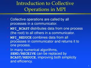
Collective Communications • allows many nodes to communicate with each other • MPI defines subroutines/functions that implement common collective modes of communication. • relieves the user of having to develop his/her own out of send/recv primitives. • Good MPI implementations should have these collective operations already optimized for the target hardware.
Some Fundamental Modes of Collective Communication • broadcast Send something from one processor to everybody • reduce Send something from everybody and combine it together on one processor • barrier Pause until everybody has encountered this barrier • scatter Take multiple pieces of data from one process and send individual pieces of it to individual processes • gather Gather individual pieces of data from individual processes and create multiple pieces of data on a single process.