Download
1 / 40
400 likes | 497 Views
Fundamentals/ICY: Databases 2013/14 WEEK 11 (relational operators & relational algebra). John Barnden Professor of Artificial Intelligence School of Computer Science University of Birmingham, UK.

E N D
Fundamentals/ICY: Databases2013/14WEEK 11(relational operators & relational algebra) John Barnden Professor of Artificial Intelligence School of Computer Science University of Birmingham, UK
Relational Operatorssee also textbooks andone part of Week-11 Addnl NotesNB: extra Maths materialnot given there
Relational algebra Defines abstract way of expressing the manipulation of tables using “relational operators”. SELECT PROJECT JOIN (various sorts) INTERSECT Use of relational algebra operators on existing tables produces new tables UNION DIFFERENCE PRODUCT ((DIVIDE)) Relational Database Operators
Select [better name would be Select-Rows] • SQL: • SELECT * FROM … WHERE … • Note: it’s the WHERE part that is actually doing the selection according to a criterion. • Relational algebra notation in Additional Notes: • Result table is C(T) where T is the given table and C is the selection criterion. • More compact than SQL notation. Avoids notation private to particular versions of particular programming languages.
Project [better name would be Select-Columns] • SQL: • SELECT …column specs … FROM … • Relational algebra notation in Additional Notes: • Result table is X(T) where T is the given table and X is the list of selected attributes (columns).
Relational Operators (continued) • Union and its All version • Intersect and its All version • Difference and its All version • The given tables must have compatible value domains.
Union, Intersection and Difference • SQL: • UNION, INTERSECT, EXCEPT (or MINUS) • UNION ALL, INTERSECT ALL, EXCEPT (or MINUS) ALL • Relational algebra notation for the non-All cases: • Result tables are T1T2, T1T2 and T1 T2 where T1 and T2 are the given tables. • Maths of relations: • Result relations: R1 R2, R1 R2 and R1\ R2 (or R S) in the non-ALL cases. where R1and R2 are the relations in the given tables. • Problem: relations don’t account for duplicates of rows, so don’t handle the ALL versions.
Some “Math’l Relation Operations”:Set Operations Applied to Relations Union of relations R and S: R S = the set of tuples that are in R or S (or both). NB: no repetitions created! Intersection of relations R and S: R S = the set of tuples that are in both R and S. Difference of relations R and S: R S = R \ S = the set of tuples that are in R but not S.
Mathematical Relation Operations: a contrast to Relational Operators The math’l operations do NOT themselves require R and S to have similar tuples in order to be well-defined. E.g., R could be binary and on integer sets, S could be ternary and on character-string sets. But the corresponding relational operators do require the tables to have the same shape (same number of columns, same domains for corresponding columns).
Relational Operators (continued) • Join (various types) • Allows us to join related rows from two or more tables • It’s an important feature of the relational database idea • Joining has been implicitly important in some of the Additional Notes, because of the use of mutli-table queries and the use of WHERE to test for attribute equality between tables.
Relational Operators (continued) • Productor Cross Join • Yields a table containing all concatenations of whole rows from first given table with whole rows from second given table.
Product or Cross-Join If second table also had a PRICE attribute, then the product would have a Table1.PRICE attr. and a Table2.PRICE attr.
So, I want … • ….. to define the non-standard notion of “flattened Cartesian product” of two relations R and S. • I will notate it by the symbol (underlined multiplication symbol). • R S = the set of tuples that are the concatenations of members of R and members of S. • E.g., if <a,b,c> is in R and <d,e,f> is in S, • then <a,b,c> o <d,e,f>=<a,b,c,d,e,f> is in R S. • A standard alternative notation: R o S (i.e., just “coerce” the concatentaion symbol used for tuples).
Contd. • If A is the People relation and B is the Organizations relation, and • A has members of form E156, ‘Sam’, ‘Finks’, I678> and • B has members of form I459, ‘Dell’, ‘UK’> • THEN • A B has members of form • E156, ‘Sam’, ‘Finks’, I678>, I459, ‘Dell’, ‘UK’> > • BUT • A B has members of form • E156, ‘Sam’, ‘Finks’, I678, I459, ‘Dell’, ‘UK’>
Product or Cross Join (continued) • SQL: • SELECT * FROM …two [or more] tables … • NB: it’s the mere listing of the tables that does the Product, but it’s possible also to write: • SELECT * FROM T1 CROSS JOIN T2 CROSS JOIN ... • Relational algebra notation: • Result table is T1 T2 where T1 and T2 are the given tables. • Maths of relations: • Result relationis R1 R2 where R1and R2 are the relations in the given tables. • Problem: relations don’t account for duplicates of rows.
Natural Join • SQL: • SELECT …all the attributes but including only one version of each shared one … FROM T1, T2 WHERE … explicit condition of equalities for ALL the shared attributes ... • SELECT * FROM T1 NATURAL JOIN T2; • Instead of using *, can choose columns, and can add a WHERE • Relational algebra notation: • Result table is T1T2 where T1 and T2 are the given tables. is the “bow tie” symbol.
Correspondence to your SQL experience: • SELECT sid, office FROM staff, lecturing • WHERE staff.sid = lecturing.sid; • Does a natural join (because sid is the only shared attribute) followed by a projection onto sid, office. • SELECT sid, office FROM staff, lecturing • WHERE staff.sid = lecturing.sid AND year > 2001; • In effect, does a natural join followed by a further (row) selection followed by a projection. • SELECT sid, office • FROM staff NATURAL JOIN lecturing • WHERE year > 2001; • Does same thing.
Natural Join (contd) • The common attributes or columns are called the join attributes or columns): just the AGENT_CODE attribute in above example • Can be thought of as the result of a three-stage process: • the PRODUCT of the tables is created • a SELECT is performed on the resulting table to yield only the rows for which the join-attribute values (e.g. AGENT_CODE values) are equal • a PROJECT is now performed to yield a single copy of each join attribute, thereby eliminating duplicate columns
Natural Join, Step 1: PRODUCT Note the two AGENT_CODE columns
Natural Join, Step 2: SELECTto get equal agent codes in each row
Natural Join (continued) • A row in one of the given tables that does not match any row in the other given table on the join attributes does not lead to a row in the result table. • Note that if the two tables have no attributes in common, then every row of each table trivially matches every row of the other table! • So in this case the result is the PRODUCT (CROSS JOIN) of the two tables!!
Other Forms of Join • Equijoin • Links tables on the basis of an equality condition that compares SPECIFIED attributesof each table, rather than automatically taking the common attributes. • Result does not eliminate duplicate columns that are not involved in the join condition. • Theta join • Like equijoin but using a non-equality join condition. • Outer joins (left, right, and full) • Equijoin or theta join plus unmatched rows from left table, right table or both, padding them out with NULLs to fit the result table.
Equijoin and Theta Join (continued) • SQL: • SELECT * FROM T1, T2 WHERE … explicit join condition, stating (non)equality of the CHOSEN attributes ... • SELECT * FROM T1 JOIN T2 ON … such a condition … • SELECT * FROM T1 JOIN T2 USING (… some common attribs …) • [for equijoin only] • Possible Rel’l Algebra notation (not in Addl Nts): • T1CT2 where C is the join condition.
Outer Join • of CUSTOMER and AGENT, using equal AGENT_CODE • Left outer • Uses all the rows in the CUSTOMER table, by doing equijoin on AGENT_CODE but also including NON-matching CUSTOMER rows. • Right outer • Uses all the rows in the AGENT table, doing equijoin on AGENT_CODE but also including NON-matching AGENT rows. • Full outer • Using all the rows in the AGENT and CUSTOMER tables, doing equijoin on AGENT_CODE but also including NON-matching rows from each table. • = Union of Left Outer Join result and Right Outer Join result.
Left Outer Join Same as an equijoin with the addition of the “extra”, last, row shown above
Right Outer Join: Full Outer Join: Would have the “extra” row of this table as well as the extra row of the Left Outer Join table
Outer Joins (continued) • SQL: • SELECT * FROM T1, T2 WHERE … explicit join condition … • UNION … a SELECT expression that gets the extra LEFT rows • UNION … a SELECT expression that gets the extra RIGHT rows • SELECT * FROM T1 LEFT/RIGHT/FULL JOIN T2 • USING (… some shared attribs…) / ON … explicit join cond… • Relational algebra notation: • Variants of bow tie symbol.
Note on SQL Outer Join Queries • Can do your own extra projection (= attrib selection) in the SELECT, and can add a WHERE. • E.g.: • SELECT …attribs … FROM T1 LEFT JOIN T2 • USING (… some shared attribs …) WHERE … ;
Towards the DIVIDE operation • It’s analogous to the “integer division” of an integer T by an integer S, included in many programming languages. • T div S = the largestintegerQ such that • S Q T • So 7 div 3 = 2.
DIVIDE operation on DB tables Simplest case: 2-col table by 1-col table T S Q The only value of LOC that is associated in T with both values ‘A’ and ‘B’ of CODE is 5.
Divide • DIVIDE T by S: the attributes X1 … XM of table S must be some but not all of those of T’s. • Gives a table Q having the remaining attributes Y1 … YN of T. • Q holds the values of Y1 … YN that T associates with every row (X1 … XM) in S. • So the rows of the Product of S with Q form a subset of the rows (suitably re-ordered) of T, and Q is maximal in this respect (i.e., adding further rows to Q would stop the Product’s rows all being in T) • So Q is the largest table such that • S Q T • using to mean: has some or all rows of.
Divide (continued) • SQL: • Not standardly included. Effect can be simulated. • possible Relational Algebra notation (not in Add’l Notes): • T2 T1 • Maths of relations: • Result relationRcould be described as • themaximalset R of tuples such that R1 R R2 • where R1 and R2 are the relations in the given tables.