Download
1 / 25
260 likes | 438 Views
Refresher: Vector and Matrix Algebra. Mike Kirkpatrick Department of Chemical Engineering FAMU-FSU College of Engineering. Outline. Basics: Operations on vectors and matrices Linear systems of algebraic equations Gauss elimination Matrix rank, existence of a solution Inverse of a matrix

E N D
Refresher:Vector and Matrix Algebra Mike Kirkpatrick Department of Chemical Engineering FAMU-FSU College of Engineering
Outline • Basics: • Operations on vectors and matrices • Linear systems of algebraic equations • Gauss elimination • Matrix rank, existence of a solution • Inverse of a matrix • Determinants • Eigenvalues and Eigenvectors • applications • diagonalization more
Outline cont’ • Special matrix properties • symmetric, skew-symmetric, and orthogonal matrices • Hermitian, skew-Hermitian, and unitary matrices
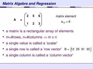
Matrices • A matrix is a rectangular array of numbers (or functions). • The matrix shown above is of size mxn. Note that this designates first the number of rows, then the number of columns. • The elements of a matrix, here represented by the letter ‘a’ with subscripts, can consist of numbers, variables, or functions of variables.
Vectors • A vector is simply a matrix with either one row or one column.A matrix with one row is called a row vector, and a matrix with one column is called a column vector. • Transpose: A row vector can be changed into a column vector and vice-versa by taking the transpose of that vector. e.g.:
Matrix Addition • Matrix addition is only possible between two matrices which have the same size. • The operation is done simply by adding the corresponding elements. e.g.:
Matrix scalar multiplication • Multiplication of a matrix or a vector by a scalar is also straightforward:
Transpose of a matrix • Taking the transpose of a matrix is similar to that of a vector: • The diagonal elements in the matrix are unaffected, but the other elements are switched. A matrix which is the same as its own transpose is called symmetric, and one which is the negative of its own transpose is called skew-symmetric.
Matrix Multiplication • The multiplication of a matrix into another matrix not possible for all matrices, and the operation is not commutative: AB ≠ BA in general • In order to multiply two matrices, the first matrix must have the same number of columns as the second matrix has rows. • So, if one wants to solve for C=AB, then the matrix A must have as many columns as the matrix B has rows. • The resulting matrix C will have the same number of rows as did A and the same number of columns as did B.
Matrix Multiplication • The operation is done as follows: using index notation: • for example:
Linear systems of equations • One of the most important application of matrices is for solving linear systems of equations which appear in many different problems including electrical networks, statistics, and numerical methods for differential equations. • A linear system of equations can be written: a11x1 + … + a1nxn = b1 a21x1 + … + a2nxn = b2 : am1x1 + … + amnxn = bm • This is a system of m equations and n unknowns.
Linear systems cont’ • The system of equations shown on the previous slide can be written more compactly as a matrix equation: Ax=b • where the matrix A contains all the coefficients of the unknown variables from the LHS, x is the vector of unknowns, and b a vector containing the numbers from the RHS
Gauss elimination • Although these types of problems can be solved easily using a wide number of computational packages, the principle of Gaussian elimination should be understood. • The principle is to successively eliminate variables from the equations until the system is in ‘triangular’ form, that is, the matrix A will contain all zeros below the diagonal.
Gauss elimination cont’ • A very simple example: -x + 2y = 4 3x + 4y =38 first, divide the second equation by -2, then add to the first equation to eliminate y; the resulting system is: -x + 2y = 4 -2.5x = -15 x = 6 y = 5
Matrix rank • The rank of a matrix is simply the number of independent row vectors in that matrix. • The transpose of a matrix has the same rank as the original matrix. • To find the rank of a matrix by hand, use Gauss elimination and the linearly dependant row vectors will fall out, leaving only the linearly independent vectors, the number of which is the rank.
Matrix inverse • The inverse of the matrix A is denoted as A-1 • By definition, AA-1 = A-1A = I, where I is the identity matrix. • Theorem: The inverse of an nxn matrix A exists if and only if the rank A = n. • Gauss-Jordan elimination can be used to find the inverse of a matrix by hand.
Determinants • Determinants are useful in eigenvalue problems and differential equations. • Can be found only for square matrices. • Simple example: 2nd order determinant
3rd order determinant • The determinant of a 3X3 matrix is found as follows: • The terms on the RHS can be evaluated as shown for a 2nd order determinant.
Some theorems for determinants • Cramer’s: If the determinant of a system of n equations with n unknowns is nonzero, that system has precisely one solution. • det(AB)=det(BA)=det(A)det(B)
Eigenvalues and Eigenvectors • Let A be an nxn matrix and consider the vector equation: Ax = x • A value of for which this equation has a solution x≠0 is called an eigenvalue of the matrix A. • The corresponding solutions x are called the eigenvectors of the matrix A.
Solving for eigenvalues Ax=x Ax - x = 0 (A- I)x = 0 • This is a homogeneous linear system, homogeneous meaning that the RHS are all zeros. • For such a system, a theorem states that a solution exists given that det(A- I)=0. • The eigenvalues are found by solving the above equation.
Solving for eigenvalues cont’ • Simple example: find the eigenvalues for the matrix: • Eigenvalues are given by the equation det(A-I) = 0: • So, the roots of the last equation are -1 and -6. These are the eigenvalues of matrix A.
Eigenvectors • For each eigenvalue, , there is a corresponding eigenvector, x. • This vector can be found by substituting one of the eigenvalues back into the original equation: Ax = x : for the example: -5x1 + 2x2 = x1 2x1 – 2x2 = x2 • Using =-1, we get x2 = 2x1, and by arbitrarily choosing x1 = 1, the eigenvector corresponding to =-1 is: and similarly,
Special matrices • A matrix is called symmetric if: AT = A • A skew-symmetric matrix is one for which: AT = -A • An orthogonal matrix is one whose transpose is also its inverse: AT = A-1
Complex matrices • If a matrix contains complex (imaginary) elements, it is often useful to take its complex conjugate. The notation used for the complex conjugate of a matrix A is: • Some special complex matrices are as follows: Hermitian: T = A Skew-Hermitian: T = -A Unitary: T = A-1