Download
1 / 56
560 likes | 708 Views
Chapter9 Sorting(1). Outline. introduction Sorting Networks Bubble Sort and its Variants. Introduction. Sorting is the most common operations performed by a computer Internal or external Comparison-based Θ( nlog n ) and non comparison-based Θ(n). background.

E N D
Outline • introduction • Sorting Networks • Bubble Sort and its Variants
Introduction • Sorting is the most common operations performed by a computer • Internal or external • Comparison-based Θ(nlogn) and non comparison-based Θ(n)
background • Where the input and output sequence are stored? • stored on one process • distributed among the process • Useful as an intermediate step • What’s the order of output sequence among the processes? • Global enumeration
How comparisons are performed • Compare-exchange is not easy in parallel sorting algorithms • One element per process • Ts+Tw, Ts>>Tw => poor performance
How comparisons are performed (contd’) • More than one element per process • n/p elements, Ai <= Aj • Compare-split, (ts+tw*n/p)=> Ɵ(n/p)
Outline • introduction • Sorting Networks • Bitonic sort • Mapping bitonic sort to hypercube and mesh • Bubble Sort and its Variants
Sorting Networks Ɵ(log2n) • Key component: Comparator • Increasing comparator • Decreasing comparator
A typical sorting network • Depth: the number of columns it contains • Network speed is proportional to it
Bitonic sort: Ɵ(log2n) • Bitonic sequence <a0,a1,…,an> • Monotonically increasing then decreasing • There exists a cyclic shift of indices so that the above satisfied • EG: 8 9 2 1 0 4 5 7 • How to rearrange a bitonic sequence to obtain a monotonic sequence? • Let s= <a0,a1,…,an> is a bitonic sequence • s1 ,s2are bitonic • every element of s1 are smaller than every element of s2 • Bitonic-split; bitonic-merge=>bitonic-merging network or
Bitonic merging network • Logncolumn
Sorting n unordered elements • Bitonic sort, bitonic-sorting network • d(n)=d(n/2)+logn => d(n)=Θ(log2n)
How to map Bitonic sort to a hypercube ? • One element per process • How to map the bitonic sort algorithm on general purpose parallel computer? • Process <=> a wire • Compare-exchange function is performed by a pair of processes • Bitonicis communication intensive=> considering the topology of the interconnection network • Poor mapping => long distance before compare, degrading performance • Observation: • Communication happens between pairs of wire which have 1 bit different
Bitonic sort algorithm on 2d processors • Tp=Θ(log2n), cost optimal to bitonic sort
A block of elements per process case • Each processor has n/p elements • S1: Think of each process as consisting of n/p smaller processes • Poor parallel implementation • S2: Compare-exchange=> compare-split:Θ(n/p)+Θ(n/p) • The different: S2 initially sorted locally • Hypercube • mesh
Performance on different Architecture • Either very efficient nor very scalable, since the sequential algorithm is sub optimal
Outline • introduction • Sorting Networks • Bubble Sort and its Variants
Bubble sort • O(n2) • Inherently sequential
Odd-even transposition • N phases, each Θ(n) comparisons
Parallel formulation • O(n)
Shellsort • Drawback of odd-even sort • A sequence which has a few elements out of order, still need Θ(n2) to sort. • idea • Add a preprocessing phase, moving elements across long distance • Thus reduce the odd and even phase
Conclusion • Sorting Networks • Bitonic network • Mapping to hypercube and mesh • Bubble Sort and its Variants • Odd-even sort • Shell sort
Outline • Issues in Sorting • Sorting Networks • Bubble Sort and its Variants • Quick sort • Bucket and Sample sort • Other sorting algorithms
Quick Sort • Feature • Simple, low overhead • Θ(nlogn) ~ Θ(n2), • Idea • Choosing a pivot, how? • Partitioning into two parts, Θ(n) • Recursively solving two sub-problems • complexity • T(n)=T(n-1)+ Θ(n)=> Θ(n2) • T(n)=T(n/2)+Θ(n)=>Θ(nlogn)
Parallelizing quicksort • Solution 1 • Recursive decomposition • Drawback: partition handled by single process, Ω(n). Ω(n2) • Solution 2 • Idea: performing partition parallelly • we could partition an array of size n into two smaller arrays in time Θ(1) by using Θ(n) processes • how? • CRCW PRAM, Shard-address, message-passing model
Parallel Formulation for CRCW PRAM –cost optimal • assumption • n elements, n process • write conflicts are resolved arbitrarily • Executing quicksort can be visualized as constructing a binary tree
algorithm 1. procedure BUILD TREE (A[1...n]) 2. begin 3. for each process i do 4. begin 5. root := i; 6. parenti := root; 7. leftchild[i] := rightchild[i] := n + 1; 8. end for 9. repeat for each process i ≠ root do 10. begin 11. if (A[i] < A[parenti]) or (A[i]= A[parenti] and i <parenti) then 12. begin 13. leftchild[parenti] :=i ; 14. if i = leftchild[parenti] then exit 15. else parenti := leftchild[parenti]; 16. end for 17. else 18. begin 19. rightchild[parenti] :=i; 20. If i = rightchild[parenti] then exit 21. else parenti := rightchild[parenti]; 22. end else 23. end repeat 24. end BUILD_TREE • Assuming balanced tree: • Partition distribute • To all process O(1) • Θ(logn) * Θ(1)
Parallel Formulation for Shared-Address-Space Architecture • assumption • N element, p processes • Shared memory • How to parallelize? • Idea of the algorithm • Each process is assigned a block • Selecting a pivot element, broadcast • Local rearrangement • Global rearrangement=> smaller block S, larger block L • redistributing blocks to processes • How many? • Until breaking the array into p parts
Example How to compute the location?
Analysis • Assumption • Pivot selection results in balanced partitions • Logpsteps • Broadcasting Pivot Θ(logp) • Locally rearrangement Θ(n/p) • Prefix sum Θ(log p) • Global rearrangement Θ(n/p)
Parallel Formulation for Message Passing Architecture • Similar to shared-address architecture • Different • Array distributed to p processes
Pivot selection • Random selection • Drawback: bad pivot lead to significant performance degradation • Median selection • Assumption: the initial distribution of elements in each process is uniform
Outline • Issues in Sorting • Sorting Networks • Bubble Sort and its Variants • Quick sort • Bucket and Sample sort • Other sorting algorithms
Bucket Sort • Assumption • n elements distributed uniformly over [a, b] • Idea • Divided into m equal sized subinterval • Element replacement • Sorted each one • Θ(nlog(n/m)) => Θ(n) • Compare with QuickSort
Parallelization on message passing architecture • N elements, p processes=> p buckets • Preliminary idea • Distributing elements n/p • Subinterval, elements redistribution • Locally sorting • Drawback: the assumption is not realistic => performance degradation • Solution: • Sample sorting => splitters • Guarantee elements < 2n/m
analysis • Distributing elements n/p • Local sort & sample selection Θ(p) • Sample combining Θ(P2),sortingΘ(p2logp), global splitter Θ(p) • elements partitioning Θ(plog(n/p)), redistribution O(n)+O(plogp) • Locally sorting