Download

1 / 78
780 likes | 959 Views
Phylogenetic Analysis. Review of Linux. ls cd mkdir less cp mv cat pwd >. Perl. Variables $DNA="A"; @DATA=('A', 'B'); %TABLE=(A=>'A', N=>'[AC]',); Statements print length open close substr push pop shift unshift. #!/usr/bin/perl –w $word = 'MNIDDKL';

E N D
Review of Linux • ls • cd • mkdir • less • cp • mv • cat • pwd • >
Perl • Variables • $DNA="A"; • @DATA=('A', 'B'); • %TABLE=(A=>'A', N=>'[AC]',); • Statements • print • length • open • close • substr • push • pop • shift • unshift
#!/usr/bin/perl –w $word = 'MNIDDKL'; if($word eq 'QSTVSGE') { print "QSTVSGE\n"; } elsif($word eq 'MRQQDMISHDEL') { print "MRQQDMISHDEL\n"; } elsif ( $word eq 'MNIDDKL' ) { print "MNIDDKL-the magic word!\n"; } else { print "Is \”$word\“ a peptide?\n"; } exit;
$x = 10; $y = -20; if ($x <= 10) { print "1st true\n";} if ($x > 10) {print "2nd true\n";} if ($x <= 10 || $y > -21) {print "3rd true\n";} if ($x > 5 && $y < 0) {print "4th true\n";} if (($x > 5 && $y < 0) || $y > 5) {print "5th true\n";}
$position = 0; while ( $position < length $DNA) { $base = substr($DNA, $position, 1); if ( $base eq 'C' or $base eq 'G') { ++$count_of_CG; } $position++; } for ( $position = 0 ; $position < length $DNA ; ++$position ) { $base = substr($DNA, $position, 1); if ( $base eq 'C' or $base eq 'G') { ++$count_of_CG; } }
Converting Formats • Don’t re-compute your MSA if it is not in the right format • Convert your file using one of the online conversion tools • The 3 most popular reformatting utilities: • Fmtseq The most complete • RESDSEQ Very popular and robust • SeqCheck Can clean FASTA sequences
Editing your MSA • If your MSA looks bad . . . • Don’t torture the online server • Edit the MSA yourself locally • Never, ever, ever (ever) use a standard word processor • Always use a dedicated MSA editor • The most popular online tool is Jalview • You can get it at www.jalview.org
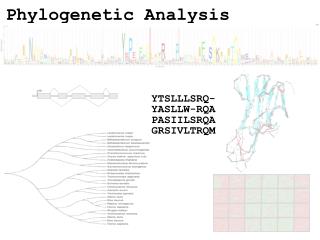
MSA => LOGO Graph • A LOGO graph summarizes an MSA • Tall letters indicate highly conserved positions • Short letters indicate poorly conserved positions • LOGO graphs are ideal for identifying conserved patterns • weblogo.berkeley.edu/
Human Evolutionary Tree (cont’d) http://www.mun.ca/biology/scarr/Out_of_Africa2.htm
Human Migration Out of Africa 1. Yorubans 2. Western Pygmies 3. Eastern Pygmies 4. Hadza 5. !Kung 1 2 3 4 5 http://www.becominghuman.org
Reading Your Tree • There’s a lot of vocabulary in a tree • Nodes correspond to common ancestors • The root is the oldest ancestor • Often artificial • Only meaningful with a good outgroup • Trees can be un-rooted • Branch lengths are only meaningful when the tree is scaled • Cladograms are often scaled • Phenograms are usualy unscaled
Rooted and Unrooted Trees • In the unrooted tree the position of the root (“oldest ancestor”) is unknown. Otherwise, they are like rooted trees
Orthology and Paralogy 直系(垂直)同源和旁系(平行)同源 • Orthologous genes • Separated by speciation • Often have the same function • Paralogous genes • Separated by duplications • Can have different functions • In the graph: • A is paralogous with B • A1 is orthologous with A2
Which Sequences ? • Orthologous sequences • Produce a species tree • Show how the considered species have diverged • Paralogous sequences • Produce a gene tree • Show the evolution of a protein family
Building the Right MSA • Your MSA should have as few gaps as possible. Most time should remove columns with gaps. • Some variability but not too much! • Some conservation but not too much!
Building the Right Tree • There are three types of tree-reconstruction methods • Distance-based methods • Statistical methods • Parsimony methods • Statistical methods are the most accurate • Maximum likelihood of success • Bayesian methods • Statistical methods take more time • Limited to small datasets
j i Distance in Trees: an Exampe d1,4 = 12 + 13 + 14 + 17 + 12 = 68
Compute a Distance Matrix Evolutionary Distance - number of substitutions per 100 amino acids (for proteins) or nucleotides (for DNA) A C T G T A G G A A T C G C A A T G A A A G A A T C G C 3 observed changes A C T G T A G G A A T C G C A C T G C A G G A A T A G C A A T G A A A G A A T C G C 6 actual changes
j i Edit Distance vs Tree Distance d1,4 = 12 + 13 + 14 + 17 + 12 = 68 D1,4 may be smaller than 68, as some changes may not be observed
Fitting Distance Matrix • Given n species, we can compute the n x n distance matrixDij • Evolution of these genes is described by a tree that we don’t know. • We need an algorithm to construct a tree that best fits the distance matrix Dij
Tree reconstruction for any 3x3 matrix is straightforward We have 3 leaves i, j, k and a center vertex c Reconstructing a 3 Leaved Tree Observe: dic + djc = Dij dic + dkc = Dik djc + dkc = Djk
dic + djc = Dij + dic + dkc = Dik 2dic + djc + dkc = Dij + Dik 2dic + Djk = Dij + Dik dic = (Dij + Dik – Djk)/2 Similarly, djc = (Dij + Djk – Dik)/2 dkc = (Dki + Dkj – Dij)/2 Reconstructing a 3 Leaved Tree(cont’d)
Additive Distance Matrices Matrix D is ADDITIVE if there exists a tree T with dij(T) = Dij NON-ADDITIVE otherwise
The Four Point Condition (cont’d) Compute: 1. Dij + Dkl, 2. Dik + Djl, 3. Dil + Djk 2 3 1 2 and 3 represent the same number: the length of all edges + the middle edge (it is counted twice) 1 represents a smaller number: the length of all edges – the middle edge
The Four Point Condition: Theorem • The four point condition for the quartet i,j,k,l is satisfied if two of these sums are the same, with the third sum smaller than these first two • Theorem : An n x n matrix D is additive if and only if the four point condition holds for every quartet 1 ≤ i,j,k,l ≤ n
Distance Based Phylogeny Problem • Goal: Reconstruct an evolutionary tree from a distance matrix • Input: n x n distance matrix Dij • Output: weighted tree T with n leaves fitting D • If D is additive, this problem has a solution and there is a simple algorithm to solve it
Find neighboring leavesi and j with parent k Remove the rows and columns of i and j Add a new row and column corresponding to k, where the distance from k to any other leaf m can be computed as: Using Neighboring Leaves to Construct the Tree Dkm = (Dim + Djm – Dij)/2 Compress i and j into k, iterate algorithm for rest of tree
Finding Neighboring Leaves • To find neighboring leaves we simply select a pair of closest leaves.
Finding Neighboring Leaves • To find neighboring leaves we simply select a pair of closest leaves. • WRONG
Finding Neighboring Leaves • Closest leaves aren’t necessarily neighbors • i and j are neighbors, but (dij= 13) > (djk = 12) • Finding a pair of neighboring leaves is • a nontrivial problem!
Neighbor Joining Algorithm • In 1987 Naruya Saitou and Masatoshi Nei developed a neighbor joining algorithm for phylogenetic tree reconstruction • Finds a pair of leaves that are close to each other but far from other leaves: implicitly finds a pair of neighboring leaves • Advantages: works well for additive and other non-additive matrices, it does not have the flawed molecular clock assumption
Overview • Based on the current distance matrix calculate the matrix Q (defined later). • Find the pair of taxa for which has its lowest value Qij. Add a new node to the tree, joining these taxa to the rest of the tree. • Calculate the distance from each of the taxa in the pair to this new node. • Calculate the distance from each of the taxa outside of this pair to the new node. • Start the algorithm again, replacing the pair of joined neighbors with the new node and using the distances calculated in the previous step.
D Q
D Q
D Q
D(AU) =d(AB) / 2 + [r(A)-r(B)] / 2(N-2) = 1 D(BU) =d(AB) -D(AU) = 4 Tree (So far)
d(CU) = [d(AC) + d(BC) - d(AB)] / 2 = 3 d(DU) = [d(AD) + d(BD) - d(AB) ]/ 2 = 6 d(EU) = [d(AE) + d(BE) - d(AB) ]/ 2 = 5 d(FU) = [d(AF) + d(BF) - d(AB) ]/ 2 = 7 New Matrix