Download
1 / 45
450 likes | 551 Views
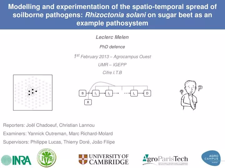
Modelling and experimentation of the spatio-temporal spread of soilborne pathogens: Rhizoctonia solani on sugar beet as an example pathosystem. Leclerc Melen. PhD defence 1 st February 2013 – Agrocampus Ouest UMR – IGEPP Cifre I.T.B. Reporters: Joël Chadoeuf, Christian Lannou

E N D
Modelling and experimentation of the spatio-temporal spread of soilborne pathogens: Rhizoctonia solani on sugar beet as an example pathosystem Leclerc Melen PhD defence 1st February 2013 – Agrocampus Ouest UMR – IGEPP Cifre I.T.B Reporters: Joël Chadoeuf, Christian Lannou Examiners: Yannick Outreman, Marc Richard-Molard Supervisors: Philippe Lucas, Thierry Doré, João Filipe
Introduction General context – current problems • 50% reduction in pesticide use (Grenelle de l’environnement Ecophyto) • Find alternatives to pesticide use • Keep crop production levels and growers’ incomes
Introduction Proposed approaches • Necessity of considering the complexity of agro-ecosystems (e.g. using system approaches) • Understand ecological and epidemiological processes involved in the dynamics of pathogens • Use ecological and epidemiological knowledge to improve pest management and design efficient crop protection strategies • Combine several controls with partial effects (there is no ‘one fits all’ solution) • SysPID Casdar Project: Reduce the impact of soilborne diseases in crop systems towards an integrated and sustainable pest management • Action n°2: Epidemiological processes in field crop systems
Introduction Soilborne disease epidemics • Soilborne diseases • Wide range of pathogenic organisms (fungi, bacteria, viruses, nematodes, protozoa) • Cause substantial damage to crops worldwide (up to 50 % of crop loss in the US (Lewis & Papaizas, 1991) ) • Pathogens often survive for many years in soils (5-7 years for Pythium) • Difficult to detect, predict and control • Epidemiology • External source of inoculum X(t) : dynamic pathogen population • Primary infections : external inoculum epidemic initiation • Secondary infections : spread of the pathogen within the crop/population Susceptible hosts Infected/Infectious hosts S I X
Rhizoctonia solani on sugar beet as an example pathosystem Introduction The host The pathogen
Introduction The host : sugar beet • The plant • Cultivated Beta vulgaris • High production of sucrose • The crop • Grown for sugar production • France is one of the largest producer (33 Mt in 2009)
Introduction The pathogen : Rhizoctonia solani • R. solani fungi • Basidiomycetes • Polyphagous saprotrophic fungi • Anastomisis Groups (AG) • R. solani AG2-2 IIIB • Parasites maize, rice, sugar beet, ginger … • Important optimal temperature range for growth • Develops late in the growing season • Infects mostly mature plants Aoyagi et al., 1998
Introduction The disease : the brown root rot disease of sugar beet
Introduction Rhizoctonia root rot disease control • Current management strategies • Think crop rotations (host & non-host crops) • Resistant varieties • Biological controls ? • Antagonists (e.g. Trichoderma fungi) • Biofumigation
Introduction Our system Visible epidemic: symptomatic plants Above-ground Hidden epidemic: Cryptic infections Source of inoculum : R. solani Temporal scale : growing season of sugar beet Spatial scale : field Belowground
Introduction Research questions and structure of the presentation • 1. How does R. solani spread in field conditions ? (Understand epidemiology of R. solani in field conditions) • 2. How to infer hidden infections from observations of the disease ? • 3. How does biofumigation affect epidemic development ? Study 1 : R. solani spread Experimentation Modelling Study 2 : Incubation period Experimentation Modelling Study 3 : Effects of biofumigation 2007 data (Motisi, 2009) Modelling
Part 1 How does R. solani spread in field conditions ?
Part 1 Pathozone concept and spread of soilborne pathogens • Difficult to asses R. solani growth in soils use of pathozone concept • “Pathozone means the region of soil surrounding a host unit within which the centre of a propagule must lie for infection of the host unit to be possible” (Gilligan, 1985) Probability of infection Placement experiment Inoculum(donor)-host(recipient) n replicates at distance x ni number of infected recipients at time t P(x,t) = ni / n Time exposed to inoculum Contact distance
Part 1 Results of the experiments (Pathozone profiles) • Field experiments in 2011 (Le Rheu) Primary inoculum (5 infested barley seeds) Secondary inoculum (an infected plant) • Localised spread (nearest neigbour plants) (Filipe et al., 2004, Gibson et al.,2006) • Infections occurs further with secondary inoculum ( Kleczkowski et al.,1997) • The fungus translocates nutrients from the parasited host to other parts of the mycelium
Part 1 Host growth may increase pathogen transmission at individual level Host-plant growth decreases the contact distance between neighbouring plants Host growth may increase pathogen transmission at individual level
Part 1 Host growth can trigger the development of epidemics Static contact distance Dynamic contact distance xcc= 11 cm Non-invasive behaviour (linear trend) Host growth can cause a switch from non-invasive to invasive behaviour xcc= 14 cm xcc= 17 cm Invasive behaviour (non-linear trend)
Part 1 Conclusion (Part 1) • First Pathozone profiles measured in a real soil • Locality of pathogen spread in field conditions • Importance of considering space : mean-field approximation/homogeneous mixing assumption may fail when predicting the spread of soilborne pathogens(Dieckmann et al., 2000 ; Filipe & Gibson, 2001) • Host growthcan trigger the development of epidemics by decreasing contact distances • Need to take into account host growth for epidemic thresholds – conditions for invasive spread of plant population by pathogens(Grassberger, 1983 ; Brown & Bolker, 2004)
Part 2 How to infer hidden infections from observations ?
Part 2 Problem
Part 2 A problem of incubation period • Time between hidden infection and appearance of detectable symptoms of pathology • Incubation period(Kern, 1956 ; Keeling & Rohani, 2008) • Incubation period distributions are often described by non-negative probability distributions with a pronounced mode(Keeling & Rohani, 2008 ; Chan & Johansson, 2012) • Incubation period data are rare …
Part 2 Compartmental models an incubation period distributions • How to describe cryptic infections with compartmental models ? • Compartmental Markovian models • The time spent in each state is exponentially distributed • In a simple SID model the incubation period is exponentially distributed • How to introduce realistic distributions in classical compartmental models ? • A tractable way: by subdividing compartments (i.e. introducing transient states) • Sum of exponentialy distributed random variables • = • Erlang (or Gamma) distributed random variable Susceptible hosts Infected/infectious hosts Detectable/symptomatic hosts Realistic distribution Distribution in classical Markovian models
Part 2 Working hypothesis and methodology • Hypothesis: the distribution (e.g. mean and range) of the incubation period is age-dependent • Methodology: • Experimental measures for various ages of infection • Statistical analysis (is Gamma distribution robust enough ?) • Build a model for age-varying distribution of the incubation period • Incorporate it into an SID compartmental model
Part 2 Experimental measures of the incubation period • Experiments • Plant inoculated with 3 infested barley seeds (inoculum) • 9 ages of plants (14, 32, 46, 60, 74, 88, 102, 116, 130 days) • For each individual the time of first above-ground symptom was recorded • At least 45 individual observations for each age distributions of the incubation period
Part 2 Raw data (results of the experiments) Inubation period calculated in degree- days
Part 2 Age-varying model of the incubation period distribution • Age by age distribution analysis Gamma distribution (general case of Erlang)can reasonably describe incubation period distributions • Age-varying model of the incubation period T(t) k : shape parameter = number of transient states (=19) λ: time dependent rate parameter • Compartmental model with realistic incubation distribution (19 transient non-symptomatic states)
Part 2 Hidden infections and observations • Simulations of cryptic epidemics (individual-based spatial model with stochastic continuous time) Infected and detectable/symptomatic individuals have different dynamics
Part 2 Conclusion (Part 2) • One of the first epidemiological model for soilborne disease with data-supported incubation period • Link hidden processes and observations of disease • Estimate rates of infections and cryptic infections from observations • Test management strategies based on the detection of symptomatic individuals • This end of the incubation period corresponds to a visual detectability • May change with other detection/survey methods, e.g. molecular techniques, remote sensing • Variability ? (soils, human error, strains, environmental conditions …)
Part 3 How does biofumigation affect epidemic development?
Part 3 Background Force of infection • Previous work • The effect of biofumigation on the root rot disease has been analysed using a simple epidemiological model(Motisi, 2009 ; Motisi et al., 2012) • Observations of symptomatic plants for 3 treatments : • 1) without control, 2) with complete biofumigation, 3) with partial biofumigation • Biofumigation affects mostly primary infections • Biofumigation can affect secondary infections with a variable pattern
Part 3 Aim of the current study • Integratenew epidemiological knowledge and data • Improve existing epidemiological models • Re-analyse the effects of biofumigation • Investigate thevariability of epidemics to estimate uncertainty in the outcome of treatments
Part 3 Improved epidemiological model : epidemic predictions • Spatial individual-based model with stochastic spread of the pathogen • Spatial component : better description of epidemics • Stochastic model : introduce variability in outcomes predictions of uncertainty Stochastic infections Rate of primary infection Rate of secondary infection
Part 3 Estimate parameter for each treatment from observations of disease • Introduce a more realistic incubation period for inferring epidemiological parameters • Statistical inferrence of spatio-temporal can be difficult and time consuming… • Estimate spatial rates of infection using a semi-spatial model(Filipe et al., 2004) • Localized spread of infections (see Part 1) • Pair approximation (Matsuda et al., 1992 ; Filipe & Gibson, 1998 ; van Baalen, 2000) • Need to describe the dynamics of all pairs of the system (i.e. SS, SI II for an SI model) • Tractability : necessity to simplify the incubation period…
Part 3 Model fitting and estimated rates of infection Rate of primary infection Symptomatic plants (2007 data) Rate of secondary infection Biofumigation reduced rates of primary and secondary infection in this trial (2007)
Part 3 Spatial model predictions Distributions of infected plants at harvest (%) • Biofumigation allows a partial control of epidemics • Biofumigation seems to reduce the uncertainty in epidemic outcome • Marginal differences between partial and complete biofumigation in 2007
Part 3 Conclusion (Part 3) • Analyses are consistent with previous results on the effect of biofumigation on the spread of R. solani, but • We predict less primary infections and more secondary infections than in the previous study • New vision of epidemic : different disease progress curves • Biofumigation seems to reduce the uncertainty in epidemic outcome • Take these results with care • More statistical analyses are required to assess model fitting and conclude on the effects of treatments on epidemic development • Assess the effects of incubation period simplification – Pairwise vs temporal model … • Isotropic space (may overestimate epidemics ?) • Re-analyse 2008 data
General conclusion Soilborne disease epidemics • This work provide insights into root rot disease epidemics • spread of R. solani • incubation period • Data-supported studies – field experiments • We still need to improve knowledge on the epidemiology of this disease • May apply to others pathosystems : perennial and non-perennial plants
General conclusion Control of soilborne disease epidemics • Biofumigation • partial control of the root rot disease (Motisi et al., 2009 , 2010, 2012) • can reduce the uncertainty in epidemic outcome • This work points out important epidemiological parameters for disease management • Design and test new strategies Plant growth use crop mixing, precise key phenological stages to select for resistances Incubation period improve disease survey Locality of pathogen spread optimize the effects of treatments, use local treatments ? • Combine partial controls (new and conventional) improve the control of epidemics • Models may help to test disease management strategies
General conclusion Perspectives • Mutltiple perspectives (theoretical, applied, epidemiological, ecological…) • Consider main environmental parameters (temperature, moisture) • Investigate pathogen dynamic at the crop rotation scale • Understand ecological functionning of soils (pathogenic and non pathogenic communities)
Merci… • Doug Bailey • Philipe Lucas – Thierry Doré – João Filipe • Françoise Montfort • Les anciens membres de l’équipe EPSOS • UMR IGEPP • Les Unités Expérimentales de Dijon et de Le Rheu • L’Institut Technique de la Betterave • Christian Lannou – Joël Chadoeuf – Marc Richard Molard – Yannick Outreman (jury) • Pauline Ezanno – Marie Gosme – Christian Steinberg – Agnès Champeil – Étienne Rivot (comité de thèse) • Chris Gilligan et l’Epidemiology and Modelling Group • Les membres du projet Casdar SysPID • Le portakabin (qui a eu chaud…) • Et tous ceux qui m’ont supporté… Mon bureau…avant-hier
Introduction Evolution of symptoms
Introduction The pathogen: R. solani Rate of primary infection Rate of secondary infection Rates of infection and pathozones Pathozones P(x,t) x: contact distance t: time of exposure Infer parameters from pair experiment data ninf: number of infected recipients ntot: number of replicates (25)
Part 2 Incubation period ? • Periods in Natural history of disease in a host – these are incorporated as compartments in epidemiological models • Incubation period: • "time required for multiplication of a parasitic organism within a host organism up to the threshold point at which the parasite population is large enough to produce detectable symptoms of pathology“ (Kern, 1956)
Introduction Host growth and dynamic contact distances • Increase in the radius h(t) • Radial growth measured with Pepista tools (ITB) • Simple empirical model • Dynamic of the contact distance between nearest neighbours xee(t) • Static centre-centre distance xcc • Spatial population model • 30*30 square lattice • t0= 30 days • 5% infected
Part 3 First results Force of infection Previous epidemiological model Detectable/ symptomatic Infected • Assumptions • Mean field mass action/homogeneous mixing assumption • Epidemics initiated too soon • Pre-emergence damping off • Unrealistic incubation period Rate of primary infection Motisi et al., 2012