Download
1 / 50
500 likes | 626 Views
Recursion. Recall : grandparent(Pers, Gpar) :- parent(Pers, Par), parent(Par, Gpar). How to define greatgrandparents ? grandparent(Pers, GGpar) :- parent(Pers, Par), parent(Par, Gpar), parrent(Gpar, GGPar).

E N D
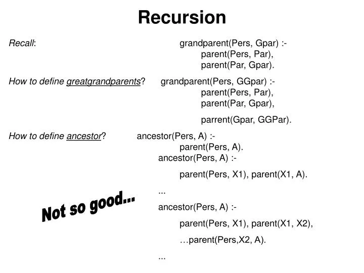
Recursion Recall: grandparent(Pers, Gpar) :- parent(Pers, Par), parent(Par, Gpar). How to define greatgrandparents? grandparent(Pers, GGpar) :- parent(Pers, Par), parent(Par, Gpar), parrent(Gpar, GGPar). How to define ancestor? ancestor(Pers, A) :- parent(Pers, A). ancestor(Pers, A) :- parent(Pers, X1), parent(X1, A). ... ancestor(Pers, A) :- parent(Pers, X1), parent(X1, X2), …parent(Pers,X2, A). ... Not so good...
Better: use Recursion ancestor(P, Anc) :- parent(P, Anc). ancestor(P, Anc) :- parent(P, Par), ancestor(Par, Anc). father(charles,philip). father(ana,george). father(philip,tom). mother(charles,ana).
Order of Clauses : Base Case first!! ancestor(P, Anc) :- parent(P, Par), ancestor(Par, Anc). ancestor(P, Anc) :- parent(P, Anc). father(charles,philip). father(ana,george). father(philip,tom). mother(charles,ana).
Paths in Graphs path(Node1, Node2) :- edge(Node1, Node2). path(Node1, Node2) :- edge(Node1, Hop), path(Hop, Node2). ?- path(a, X). X=b, X=c, X=e, X=d.
path(Node1, Node2) :- edge(Node1, Node2).Path(Node1, Node2) :- edge(Node1, Hop), path(Hop, Node2).
Terms as Data Structures • From other programming languages you know • records • structures • arrays • strings … • Prolog knows only Terms! • Terms can (and must) be used to represent all other data structures • Reminder: Terms have the following forms: • a where a is an constant • X where X is a variable • f(T1, …, Tn) where f is a functor and T1…Tn are terms • There are no type declarations in Prolog!
Records Struct person { becomes person(Name, Age, Prof). char[] Name; int age; for example char[] profession; } person(martin, 36, lawyer). Reords can be nested: person(Name, Age, Profession). profession(Type, Employer). e.g. person(john, 40, profession(pilot, qantas)).
Records Reords can be queried: person(john, 40, profession(pilot, qantas)). “What is John’s profession?” ?- person(john, _Age, Prof). “Who is John’s employer?” ?- person(john, _Age, profession(_Type, Employer)). “Who are the persons working as pilots?” ?- person(Name, _Age, profession(pilot, _Employer)).
Unification • In traditional programming we use assignments • X := Y means • “X gets the value if Y” • In logic programming there are no assignments • X = Y means • “try to make X and Y equal, but keep them as general as possible” • X=abc => X=abc • abc=X => X=abc • X=Y => no change, • but both variables identical • (as if X=_1, Y=_1) • f(a)=f(X) => X=a • f(a,Y)=f(X,X) => X=Y and X=Y=a • f(X)=X => ??????? (not permitted) • Unification computes the substitution required to make the terms equal
Unification Algorithm (Idea) Unify(C): C is a set of equations, S a substitution Initialize S to empty While C is not empty select equation c from C if c is of the from X=X then remove c from C elseif c is of the form f(X1,…,Xn)=g(Y1,…,Ym) then return false if not(f=g) or not(m=n) elseif c is of the form f(X1, …, Xn)=f(Y1, …, Yn) then replace c in C with X1=Y1, …, Xn=Yn elseif c is of the form term=X and X is a variable then replace c in C with X=term elseif c is of the form X=term and X is a variable then if term contains X then return false else (1) remove c from C, (2) replace X with t throughout C and throughout S (3) add c to S endif endif endwhile return S
Unification Exercise • abc = def ? • abc = Y ? • abc = f(Y) ? • f(abc) = f(Y) ? • g(abc) = f(Y) ? • g(abc, def, X) = g(A, Y, A) ? • g(abc, def, X) = g(A, A, A) ? • g(f(a), h(b)) = g(f(X), Y) ? <- cf. record example • g(f(a), h(b)) = g(X, k(b)) ? • X=g(X) ? • g(X,Y)=g(g(Y),a) ?
Lists (sequential collections of elements) The most important data structure in Prolog. (Partially because of the strong emphasis on recursive programming) Lists can be represented using terms Example: the list <a, b, c, d> can be represented as cons(a, cons(b, cons(c, cons(d, nil))))
Lists Lists are important enough to have a special notation [] nil [X | Y] cons(X, Y) “Y is a list” [X1, X2, …, Xn] cons(X1, cons(X2, …, cons(Xn, nil))) [X1, X2, …, Xn | Y] cons(X1, cons(X2, …, cons(Xn, Y))) Note: [X1, …, Xn | Y] is a list only if Y is a list. Its length is n + the number of elements in Y. What is the result of: [a,b] = [a|X]? [a]=[a|X]? [a]=[a, b | X]? [] = [X]?
Lists + Recursion • Lists are important, because they fit naturally into the recursive schema. The idea is: • If the list is empty (or has one element), the answer should be easy. • If the list is longer, break it up and check for the shorter lists. • Consider the test for membership in a list: • Element X is a member of the list L if • L starts with X or • the rest of X contains X • member(X, []) :- fail. • member(X, [U|V]) :- X=U. • member(X, [U|V]) :- member(X, V).
Member member(X, []) :- fail. member(X, [U|V]) :- X=U. member(X, [U|V]) :- member(X, V). Better: member(X, [X | _ ]). member(X, [_ | V]) :- member(X, V). Example: member(3, [1,2,3]) -> member(3, [2,3]) -> member(3, [3]) -> yes. Analyze: member(0, [1,2,3]) and member(X, [a,b,c]).
member/3 We can also define a predicate member(X,L,R) that checks whether an element X is in the List L and unifies R with L after removal of X member(X, [X | Rest], Rest). member(X, [_ | Rest], Rest1) :- member(X, Rest, Rest1). Analyze: member(X, [a,b], R). member(a, [a,b,a,c], R). member(c, [a,b], R). This does not achieve the desired effect, because it looses elements in front of the item that we are looking for!
member/3: Corrected member(X, [X | Rest], Rest). member(X, [F | Rest], [F | Rest1]) :- member(X, Rest, Rest1). This no longer “discards” items that are not the search element, but keeps track of them in F. The base case remains unchanged. Analyze: member(X, [a,b], R). member(a, [a,b,a,c], R). member(c, [a,b], R).
append/3 A frequently needed operation is the concatenation of two lists: append(L1, L2, L3) is defined such that L3 is the concatenation of L1 and L2 append([], L2, L2). append([X | Rest], L2, [X | Result]) :- append(Rest, L2, Result).
append/3 append([], L2, L2). append([X | Rest], L2, [X | Result]) :- append(Rest, L2, Result). What happens with the following queries? append([a,b],[c,d], Result). Yes! append(X, [b,c], [a,b,c]). Yes! append(X, Y, [a,b,c]). Yes, generates all possible solutions append(L1, [], Result). No! because first and third argument can infinitely be extended The recursion tries to shorten the first and third argument. This must eventually terminate to reach base case or to fail.
reverse/3 Here is a predicate to reverse the order of the elements in a list: reverse([], []). reverse([H | T ], L) :- reverse(T, RT), append(RT, [H], L). As defined here, reverse is hideously inefficient, Because append has to traverse the list. We will see a better solution later.
Accumulators(A better definition of reverse) reverse(X, Y) :- fast_reverse(X, [], Y). fast_reverse([], Y, Y). fast_reverse([H|T], Acc, Y) :- fast_reverse(T, [H|Acc], Y). Analyze: reverse([a,b], Y). Note: fast_reverse traverses the list only once. The second argument Acc is called an accumulator
Execution of fast_reverse • reverse([a,b,c], Y) :- fast_reverse([a,b,c], [], Y). • fast_reverse ([a,b,c], [], Y) :- fast_reverse([b,c], [a], Y). • by rule 2 • fast_reverse ([b,c], [a], Y) :- fast_reverse([c], [b,a], Y). • by rule 2 • fast_reverse ([c], [b,a], Y) :- fast_reverse([], [c,b,a], Y). • by rule 1 • fast_reverse ([], [c,b,a], [c,b,a])
Trees Trees are another very important and often used data structure, particularly binary trees (i.e. trees of degree two). struct node { struct node *left; struct node *right; elemType key; } a b c d e f g • In Prolog we use terms of structure tree(Left, Key, Right) • To represent trees, for example • tree(tree(tree(null, d, null), b, tree(null, e, null)), • tree(tree(null, f, null), c, tree(null, g, null)))
Trees Search Since a binary tree has two recursions in the data structure, a recursive predicate that traverses a tree will typically have two recursive calls. The structure of the recursion follows the structure of the data tree_member(X, tree(_, X, _)). tree_member(X, tree(L, _, _)) :- tree_member(X, L). tree_member(X, tree(_, _, R)) :- tree_member(X, R). tree_member(X, Tree) checks whether an Element X is in the Tree T
Tree Traversal • There are three different ways to traverse a tree. They are distinguished by the order in which the nodes are visited: • Inorder: left child -> node -> right child • Preorder: node -> left child -> right child • Postorder: left child -> right child -> node a Preorder(null, []). Preorder(tree(L,X,R), [X | Rest]) :- preorder(L, Left), preorder(R, Right), append(Left, Right, Rest). b c d e f g
Isomorphic Trees Two Binary Trees T1, T2 are called isomorphic If T2 can be obtained from T1 by swapping left and right subtrees. isoTree(null, null). isoTree(tree(L1, X, R1), tree(L2, X, R2)) :- isoTree(L1, L2), isoTree(R1, R2). isoTree(tree(L1, X, R1), tree(L2, X, R2)) :- isoTree(L1, R2), isoTree(R1, L2). a a iso c b b c g f d e d e f g
Visualization of Data & Predicates • As described in: G.A. Ringwood, “Predicates and Pixels”, • New Generation Computing 7 (1989): 59-80 • ...visualizes data (terms) and program (predicate) structure • in one homogeneous form... • as graphs • execution semantics defined as sub-graph substitution • The system in “Predicates and Pixels” is actually defined for a • related logic programming language called FGDC (“Flat Guarded Definite Clauses”) • defined in G.A. Ringwood, “A comparative Exploration of Concurrent Logic Languages”, • Knowledge Engineering Review 4(1989):305-332. • For the purpose of our discussion we can ignore the differences.
Example: Quicksort (with Difference Lists) we will illustrate “Predicates and Pixels” with a quicksort program that uses difference lists. Difference lists are a standard programming technique in logic programming that utilizes unification in a “tricky” form to avoid appending (because appending is a costly operation). The meaning of a difference list written “Xs\Ys” is “the list Xs disregarding the tail Ys”, e.g. [a,b,c,d,e] \ [c,d,e] = [a,b] = Xs = Ys Xs\Ys = Zs Ys\Zs = L with append(Xs,Ys,L) Xs\Zs
Standard Quicksort • quicksort([X|Xs], Ys) :- • partition(Xs, X, pair(Ls, Gs)), • quicksort(Ls, LsSorted), • quicksort(Gs, GsSorted), • append(LsSorted, [X | GsSorted], Ys). • quicksort([], []). • partition([X | Xs], P, pair([X | L1s], Gs) :- • X <= P, partition(Xs, P, L1s, Bs). • partition([X | Xs], P, pair(Ls, [X | G1s]) :- • X >= P, partition(Xs, P, pair(Ls, G1s)). • partition([], _Any, pair([], [])). • Note the inefficiency cause by using append/3.
Quicksort with Difference Lists Note that append for difference lists can simply be declared as: append_dl(Xs \ Ys, Ys \ Zs, Xs \ Zs). This can obviously be executed in constant time, but only makes sense if the tail of the first DL can be unified with the head of the second DL. ?- append_dl([a,b,c | Xs] \ Xs, [1,2] \ [], Ys) => Ys=[a,b,c,1,2] \ [] • quicksort(Xs, Ys) :- quicksort_dl(Xs, Ys \ []). • quicksort_dl([X | Xs], Y0s \ Y1s) :- • partition(Xs, X, pair(Ls, Gs)) % see last slide • quicksort_dl(Ls, Y0s \ [X | Y3s]), • quicksort_dl(Gs, Y3s \ Y1s). • quicksort_dl([], Xs\Xs).
Quicksort with Difference Lists Y0s \ Y1s Y0s \ [X | Y3s ] X = Y0s = [ X | Y3s ] = Y3s = Y1s Y3s\Y1s • quicksort(Xs, Ys) :- quicksort_dl(Xs, Ys \ []). • quicksort_dl([X | Xs], Y0s \ Y1s) :- • partition(Xs, X, pair(Ls, Gs)) % see last slide • quicksort_dl(Ls, Y0s \ [X | Y3s]), • quicksort_dl(Gs, Y3s \ Y1s). • quicksort_dl([], Xs\Xs).
Quicksort with Difference Lists (1) in the following we use: list(X, Xs) for [X | Xs] and diff(Xs, Ys) for Xs \ Ys.
Domain-Specific Data Visualization in VPLs Data Visualization only visualizes the terms used in a logic program as application specific / domain specific notations. Such programs can easily be translated into standard textual logic programs. Example: MPL (Matrix Programming Language) which incorporates a particular array notation. [6]
General Heterogeneous VPLs A Generic Schema for Data Visualization: Arbitrary Visualizations for terms can be coded into a translation module which translates the visual notation to a textual standard term. This makes domain-specific visual logic programming languages for arbitrary domains possible. Example: Finite State Automatons Exercise: Code the execution of state automatons in standard Prolog and compare to this program.
Execution of Heterogeneous VPLs Execution is achieved in three steps: (1) A preprocessor splits the program into pictures and textual program (with gaps for the pictures), (2) A customized picture parser translates the visual terms into their textual equivalents (3) The textual program and the translation of the visual terms are recombined by a standard parser, resulting in a standard (Prolog) program. (4) This program can be executed by a standard compiler. For detailed information see: Heterogeneous Visual Languages. M. Erwig and B. Meyer International IEEE Workshop on Visual Languages 1995, Darmstadt, Germany.