Download
1 / 38
380 likes | 524 Views
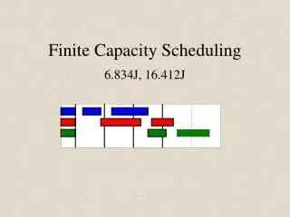
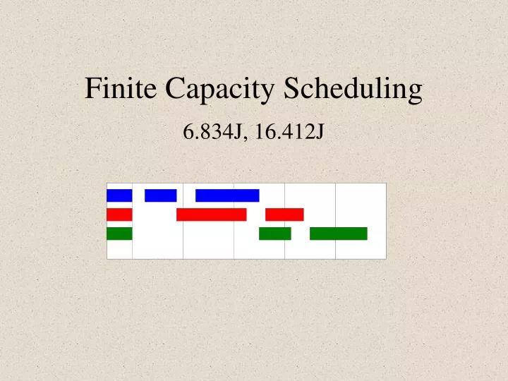
Finite Capacity Scheduling. 6.834J, 16.412J. Overview of Presentation. What is Finite Capacity Scheduling? Types of Scheduling Problems Background and History of Work Representation of Schedules Representation of Scheduling Problems Solution Algorithms Summary. Solution Algorithms.

E N D
Finite Capacity Scheduling 6.834J, 16.412J
Overview of Presentation • What is Finite Capacity Scheduling? • Types of Scheduling Problems • Background and History of Work • Representation of Schedules • Representation of Scheduling Problems • Solution Algorithms • Summary
Solution Algorithms • Dispatch Algorithms • MILP • Relation to A*, constructive constraint-based • Constructive Constraint-Based • Iterative Repair • Simulated Annealing • How A* heuristics can be used here (relaxation of deadline constraints) • Genetic Algorithms
Constructive Constraint-Based • Fox, et. al., ISIS • Best-first search with backtracking • Tasks for orders scheduled one at a time • Incrementally adds to partial schedule at each node in the search • If infeasibility is reached (constraint violation) • Backtrack to resolve constraint • Advantages • Relatively simple, can make use of standard algorithms like A* • Use of A* allows for incorporation of heuristics • Such heuristics are often used by human schedulers
Constructive (con.) • Discrete manufacturing example • Automobile assembly • Process plan:
Operation/Task Attributes • Assemble Doors • Continuous: start_time, finish_time, duration • Discrete: power_windows? • Assemble Car • Continuous: start_time, finish_time, duration • Discrete: deluxe? • Changeover • Continuous: start_time, finish_time, duration • Discrete: start_state, finish_state
Resource Requirement/Resource Attributes • Door Machine • Utilization – discrete function of time • Can be 0 or 1, depending on time in scheduling horizon • Power_windows? – discrete function of time • Can be yes or no, depending on time in scheduling horizon • Discrete functions of time represented as collection of discrete events, rather than vector with fixed time intervals • Continuous time rather than discrete time representation • Event is double of value and time • Ex. 0, 5:00 • Ex. Collection • ((0 0:00) (1 2:00) (0 6:00) (1 12:00)) • Collection supports queries of form get_value(time)
Constraints • Time • AssembleDoors.finish_time = AssembleDoors.start_time + AssembleDoors.duration • AssembleDoors.duration = 0.5 • Changeover.finish_time = Changeover.start_time + Changeover.duration • AssembleCar.finish_time = AssembleCar.start_time + AssembleCar.duration • AssembleCar.duration = 0.5 • Changeover.start_time >= AssembleDoors.finish_time • AssembleCar.start_time >= AssembleDoors.finish_time
Constraints • Resource Utilization and Capacity • For all t such that AssembleDoors.start_time <= t <= AssembleDoors.finish_time DoorMachine.utilization = 1 • For all t such that Changeover.start_time <= t <= Changeover.finish_time DoorMachine.utilization = 1 (represented by events (1 start_time) (0 finish_time) in utilization collection) - DoorMachine.utilization <= 1 (Automatically enforced by utilization collection mechanism, two start events not allowed without intervening finish event)
Constraints • Resource State • For all t such that AssembleDoors.start_time <= t <= AssembleDoors.finish_time DoorMachine.power_windows? = AssembleDoors.power_windows? (represented by events (pw? start_time) (pw? finish_time) in power_windows? collection) • For all t such that Changeover.start_time <= t < Changeover.finish_time DoorMachine.power_windows? = Changeover.start_state • At t = Changeover.finish_time DoorMachine .power_windows? = Changeover.finish_state • Represented by events (start_state start_time) (finish_state finish_time) • If Changeover.start_state != Changeover.finish_state Changeover.duration = 0.5 else Changeover.duration = 0
Algorithm Pseudocode • Instantiate tasks based on process plan and orders • One queue of tasks for each order • Loop • Pick order not yet scheduled • Loop • Pop task from queue for order • Assign task to resource • Propagate constraints • If feasible, continue • If not feasible, backtrack
Schedule Order 1 Assign tasks and propagate constraints
Schedule Order 2 Assign tasks and propagate constraints
Order 4 infeasible • Order deadline is violated • Need to backtrack
Success after two backtracks • Almost achieves schedule 2 times, then succeeds on third try • Requires search of 3 entire branches of tree
Problem with constructive approach • Search tree size: (R x O)! • R is number of resources, O is number of orders • Exponential, np complete • As shown in previous example, problems typically not encountered until last few orders are scheduled • As a result, typically searches entire branch of tree before finding out it is infeasible • Swapping to eliminate changeover requires backtracking • Results in significant amount of backtracking • Does not work for large, difficult scheduling problems • Even when heuristics are used • Even when A* is used • Partial schedule is often not a good indicator of how good schedule will be
Constructive Constraint-Based (con.) • Important disadvantage (often a show-stopper) • A simple swap of ordering of two tasks on a resource (something that human schedulers often do) may require significant backtracking • Ex. • Swapping to eliminate large changeover (asymetric TSP) requires backtracking • Unravels everything done between order 1 and n
Iterative Repair • Zweben, et. al., GERRY, Red Pepper Software • Scheduling of space shuttle ground operations • Johnston and Minton • Scheduling of Hubble space telescope • Begin with complete but possibly flawed schedule • Generate initial schedule quickly using simple dispatching • Iteratively modify to repair constraint violations, and to make more optimal • Each step in search is a repair step (single modification to complete schedule) • Results in either better or worse schedule • Hill-climbing (best-first) search • Searches space of possible complete assignments
Iterative Repair Example – Beer Scheduling • Filtering of alcoholic vs. non-alcoholic beer prior to packaging
Beer Scheduling- Operation/Task Attributes • Filtering • Continuous: start_time, finish_time, duration, size • Discrete: beer_type • Backwash • Continuous: start_time, finish_time, duration • Packaging • Continuous: start_time, finish_time, duration, size • Discrete: beer_type
Resource Requirement/Resource Attributes • Aged Beer • quantity – continuous function of time • Representation similar to discrete functions of time • Collection of (value time) doubles • Intermediate values obtained by linear interpolation • beer_type – discrete • Holding Tank • utilization – continuous function of time • beer_type – discrete function of time • Filter • beer_type - discrete function of time • Packaged Beer • quantity – continuous function of time • beer_type - discrete
Time Constraints • Filtering.duration = 0.2 * Filtering.size • Filtering.finish_time = Filtering.start_time + Filtering.duration • Changeover.finish_time = Changeover.start_time + Changeover.duration • (Note that no need for finish – start precedence constraints, falls out of resource utilization constraints)
Resource Utilization/Capacity Constraints • At t = Filtering.finish_time, Aged_beer.quantity = dec.(Aged_beer.quantity, Filtering.size) • Implemented by inserting event (decremented_size, finish_time) into quantity collection • At t = Filtering.finish_time, Holding_tank.utilization = inc.(Holding_tank.utilization, Filtering.size) • At t = Packaging.finish_time, Holding_tank.utilization = dec.(Holding_tank.utilization, Packaging.size) • For all t, Holding_tank.utilization <= 100 (gallons)
Resource State Constraints • Filtering.beer_type = Aged_beer.beer_type • Filtering.beer_type = Holding_tank.beer_type • Holding_tank.beer_type = Packaging.beer_type • At t = Changeover.start_time, if Changeover.beer_type != Holding_tank.beer_type Changeover.duration = 0.5 else Changeover.duration = 0.1 • At t = Changeover.finish_time, Holding_tank.beer_type = Changeover.beer_type
Cost • Cost based on lateness penalty • At t = due time, if (packaged_beer.quantity < required_quantity), cost = K * (required_quantity - packaged_beer.quantity)
Scheduling Decisions • Task sequence for filtering • Holding tank to use • Task size • Repair steps • Change resources (holding tank) • Change task position in sequence • Change task size • For batch processes, latter two are often equivalent
Iterative Repair Algorithm • Generate initial schedule using simple dispatching • Loop until cost acceptable • Try repair step • Propagate constraints • If reduces cost, continue • If increases cost, continue with small probability • Otherwise, retract repair step
Iterative Repair Example – Beer Scheduling • Assume holding tank capacity is 100 gallons • 3 orders each for 80 gallons alcoholic, non-alcoholic beer, interspersed as follows • (packaging tasks fixed)
Iterative Repair Example – Beer Scheduling • Simple dispatching produces following (flawed) schedule
Iterative Repair Example – Beer Scheduling • Iterative repair batches second A, NA tasks with first • Note that further batching is not possible (would need more tanks)
Iterative Repair (con.) • Disadvantage • May get stuck in local optimum (as with all local search techniques) • Can be mitigated using simulated annealing approach • Allow repair step that increases cost with some non-zero probability • Advantages • Inherently provides for rescheduling • Current schedule is initial (flawed) schedule for new requirements • Assumes new requirements not that different from old • Complete schedule available at all times • Though it may not be such a great schedule • Constraint relaxation is easy (a repair step) • Swapping tasks to reduce changeovers is easy (repair step) • A complete assignment is often more informative in guiding search than a partial assignment (Johnston and Minton)
Summary • Focus of this lecture was on generally useful techniques • Solution of real-world scheduling problems can make use of these techniques, but also, often requires use of problem specific heuristics • As with other problems, scheduling becomes easier as computers get faster (less need for problem-specific heuristics)