Download
1 / 15
160 likes | 415 Views
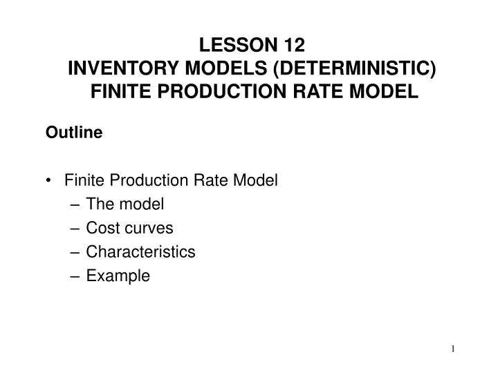
LESSON 12 INVENTORY MODELS (DETERMINISTIC) FINITE PRODUCTION RATE MODEL. Outline Finite Production Rate Model The model Cost curves Characteristics Example. Finite Production Rate . Finite production rate model is an extension of the EOQ model

E N D
LESSON 12INVENTORY MODELS (DETERMINISTIC) FINITE PRODUCTION RATE MODEL Outline • Finite Production Rate Model • The model • Cost curves • Characteristics • Example
Finite Production Rate • Finite production rate model is an extension of the EOQ model • The following assumption of the EOQ model is not used in the finite production rate model • All the quantities ordered are received at the same time (the assumption is suitable when the quantities are purchased) • An assumption in the finite production rate model • The quantity ordered is produced at an uniform rate, (the assumption is suitable when the quantities are produced) • The finite production run model is also called the Economic Production Quantity (EPQ) model
Finite Production Rate • As in the EOQ model, assume that the inventory at the beginning is zero. • The production facility is set up to produce units. If it’s optimal to produce units in the beginning, it’s also optimal to produce units next time when the inventory level reaches zero, because no cost parameter changes in between two production runs. • Therefore, like the EOQ model, the finite production rate model also has a constant order size and an inventory cycle.
Finite Production Rate • The length of the inventory cycle is the length of time over which the demand is . Thus, the length of cycle in years • In order to meet the demand (feasibility), the production rate, . Thus, for some time after the start of a new production run, the inventory level increases. The rate of increase is . The length of each production run is called the uptime and is denoted by . The uptime is the time required to produced order quantity, . So,
Finite Production Rate • If the production must be stopped before the end of the cycle in order to avoid producing more than the order quantity, units. Thus, there is a idle time or downtime in each cycle. The downtime is denoted by . • Unlike the EOQ model, the maximum inventory in the finite production rate model is not because some items are used to meet the demand before the receipt of all of the order quantity. The maximum inventory is the inventory accumulated over the uptime. Since the inventory level increases at the rate of , the maximum inventory,
Finite Production Rate • Note that the downtime demand is met entirely from the maximum inventory. Hence, downtime can also be obtained as follows: • The formula for the optimal order quantity is shown in the next slide.
Finite Production Rate = annual demand P = the production rate in units/year Q = size of each production run K = cost of setting up production h = annual holding cost per unit h´ = h(1- /P)
The Finite Production Rate Model Cost Curves Slope = 0 Annual cost ($) Total Cost Minimum total cost Holding Cost = Ordering Cost = Optimal solution, Q*,Economic Production Quantity (EPQ) Order Quantity, Q
Some Important Characteristics of the EPQ Cost Function • As in the EOQ model • The annual holding cost is the same as the annual setup cost at the EPQ • The total cost curve is flat near the EPQ • So, the total cost does not change much with a slight change in the order quantity
Example 2: Vision Optics makes microscope lens housings. Annual demand is 100,000 units per year. Assume that the product can be produced at the rate of 200,000 units per year. Each production run costs $5,000 to set up, and the variable production cost of each item is $10. The annual cost per dollar value of holding items of inventory is $0.20. Compute a. Economic production quantity
b. Cycle time c. The length of each production run (uptime per cycle) d. The length of downtime per cycle
e. The maximum inventory f. Total annual cost
READING AND EXERCISES Lesson 12 Reading: Section 4.6 , pp. 211-213 (4th Ed.) pp. 202-204 (5th Ed.) Exercise: 17 and 19, pp. 213-214 (4th Ed.), p. 204 (5th Ed.)