Download
1 / 33

E N D
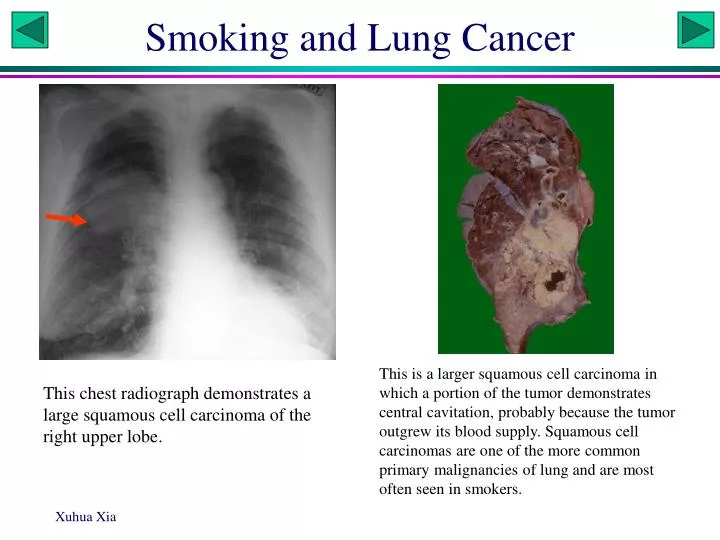
Smoking and Lung Cancer This is a larger squamous cell carcinoma in which a portion of the tumor demonstrates central cavitation, probably because the tumor outgrew its blood supply. Squamous cell carcinomas are one of the more common primary malignancies of lung and are most often seen in smokers. This chest radiograph demonstrates a large squamous cell carcinoma of the right upper lobe.
Smoking and Lung Cancer Smoker Non-smoker Lung Cancer 105 3 No Lung Cancer 99895 99996 Sub-total 100000 100000 The number of smokers and non-smokers sampled from the population
Sickness and Medication Biological and statistical questions Association between being sick and taking medicine: Taking medicine Not taking medicine Sick 990 111 Healthy 10 889 Sub-total 1000 1000 “Taking medicine” is strongly associated with “Sick”. Can we say that “Sick” is caused by “Taking medicine”?
Simpson’s paradox C. R. Charig et al. 1986. Br Med J (Clin Res Ed) 292: 879–882 Treatment A: all open procedures Treatment B: percutaneous nephrolithotomy Question: which treatment is better? Conclusion changed when a new dimension is added.
What is a Contingency Table? • A contingency table: a table of counts cross-classified according to categorical variables. • A contingency table has r rows and c columns, and is referred to as an r x c contingency table. • The simplest contingency table is a 2 x 2 table. • The most typical null hypothesis: The counts found in the rows are independent of the counts found in columns.
Contingency Tables and 2-Test • Chi-Square test is based on 2 distribution. • Chi-Square test is typically used in tests for goodness of fit, i.e., how well the observed values fit the expected values • The SAS procedure FREQ can be used to output Chi-Square statistics. • Chi-square test and Yates correction for continuity.
What is a Contingency Table? Marginal totals (Row totals) Total Marginal totals (Column totals) Cell
What is a Contingency Table? The null hypothesis: The response is independent of sex (i.e., the response is the same for both sexes). Another way of stating the null hypothesis is that the sex ratio is the same for each response category. The null hypothesis can be tested with the Chi-square test of goodness-of-fit.
X2-test of a Contingency Table? • Marginal totals • Expected frequencies (the test should be done on counts, not on proportions). • Degree of freedom • X2 value: 0 if the data is perfectly consistent with the null hypothesis. • p: the probability of obtaining the observed X2 value given that the null hypothesis is true, i.e., p(X2|H0).
X2-test of a Contingency Table? • Do hand-calculation of X2. • What is the df associated with the test? • df = (r-1)(c-1) 52 43 52 43
Chi-square Distribution The p value in chi-square test: 2 distribution is a special case of gamma distribution with = /2 and = 2. = 2 = 4 = 8 In EXCEL, p = chidist(x,DF) = 1-gammadist(x,DF/2,2,true)
Categorical Data & Associated Tests 2 by 2 contingency table Request X2-test and measures of association. Sex | Response ---------+--------+--------+ |Favour |Oppose | ---------+--------+--------+ male | 61 | 34 | ---------+--------+--------+ female | 43 | 52 | ---------+--------+--------+ Data BigIssue; input gender $ response $ wt @@; cards; Male Favour 61 Female Favour 43 Male Oppose 34 Female Oppose 52 ; proc freq; table gender*response / chisq; weight wt; run;
SAS Output GENDER RESPONSE Frequency| Percent | Row Pct | Col Pct |Favour |Oppose | Total ---------+--------+--------+ Female | 43 | 52 | 95 | 22.63 | 27.37 | 50.00 | 45.26 | 54.74 | | 41.35 | 60.47 | ---------+--------+--------+ Male | 61 | 34 | 95 | 32.11 | 17.89 | 50.00 | 64.21 | 35.79 | | 58.65 | 39.53 | ---------+--------+--------+ Total 104 86 190 54.74 45.26 100.00
SAS Output Statistic DF Value Prob ------------------------------------------------------ Chi-Square 1 6.883 0.009 Likelihood Ratio Chi-Square 1 6.927 0.008 Continuity Adj. Chi-Square 1 6.139 0.013 Mantel-Haenszel Chi-Square 1 6.847 0.009 Fisher's Exact Test (Left) 0.997 (Right) 6.50E-03 (2-Tail) 0.013 Phi Coefficient 0.190 Contingency Coefficient 0.187 Cramer's V 0.190 ---------+--------+--------+ |Favour |Oppose | ---------+--------+--------+ male | 61 | 34 | ---------+--------+--------+ female | 43 | 52 | ---------+--------+--------+
Formulas for different statistics Statistic for significance tests Measures of association: note that Phi can be used only with contingency table, otherwise the value may be greater than 1. Correlation between the two categorical variables coded in binary
2 and Measures of Association Should the two data set have the same measure of association? Should they yield the same X2 value? The same pattern as above, except that the sample size is doubled.
Sex and Hair Color GENDER COLOR | Black | Blond | Brown | Red | Total ---------+--------+--------+--------+--------+ Female | 55 | 64 | 65 | 16 | 200 ---------+--------+--------+--------+--------+ Male | 32 | 16 | 43 | 9 | 100 ---------+--------+--------+--------+--------+ Total 87 80 108 25 300 Write a SAS program to test the association between Gender and Hair Color.
SAS Output Statistic DF Value Prob ------------------------------------------------------ Chi-Square 3 8.987 0.029 Likelihood Ratio Chi-Square 3 9.512 0.023 Mantel-Haenszel Chi-Square 1 0.459 0.498 Phi Coefficient 0.173 Contingency Coefficient 0.171 Cramer's V 0.173 Sample Size = 300 The Mantel-Haenszel statistic is appropriate only when the two classification variables are on an ordinal scale (e.g., poor, average, good, excellent).
Why There Are More Blondes? • An evolutionary explanation • A genetic explanation • A simple chemical explanation • The limitation of statistics
Log-linear model • Preferred statistical tool for analyzing multi-way contingency table • Use likelihood ratio test to choose the best model • Main effects and interactions can be interpreted in a similar manner as ANOVA
Log-linear model data Disease; do Race= 1 to 2; do Disease = 1 to 2; do Loc=1 to 2; input wt @@; output; end; end; end; datalines; 44 12 38 10 28 22 20 18 ; proccatmod; weight wt; model Race*Disease*Loc=_response_ / noparm pred=freq; loglin Race|Disease|Loc @ 2; quit; • Do two races distribute similarly in the two locations? • Do races differ in their susceptibility to the disease? • Is the disease more prevalent in one location than the other? • Significant 3-way interactions (e.g., one race is more susceptible to disease in one location but less susceptible to disease in the other location)? Run and explain
Log-linear model data YeastBPS; input S1 $ S2 $ S3 $ S4 $ S5 $ S6 $ S7 $ wt; datalines; U A C U A A C 212 A A C U A A C 11 A A C U A A U 5 C A C U A A C 8 G A C U A A C 8 U A C U A A U 4 U A C U G A C 2 U A U U A A C 3 U G C U A A C 3 C G C U A A C 1 ; proccatmod; weight wt; model S1*S2*S3*S5*S7=_response_ / noparm pred=freq; loglin S1|S2|S3|S5|S7 @ 3; run;
Goodness of fit tests • Deviation of sex ratio from 1:1 • Deviation from Mendelian 3:1 ratio • Deviation from Mendelian 9:3:3:1 ratio
The spatial distribution of animals and plants has been described as random, contagious and even. We will learn some basic statistical techniques to detect these spatial patterns. Spatial Statistics
Three Distribution Patterns Random Even Contagious
Quadrat Sampling Quadrat N 1 2 2 2 3 3 4 0 5 6 . . . . 100 1 Mean Variance
Three Probability Distributions • Poisson distribution (random distribution)2 = • Binomial distribution (even distribution)2 < • Negative binomial distribution (contagious distribution)2 >
Random Distribution Conclusion: The spatial distribution of the species does not deviate significantly from random distribution. Var = [14*(0-1.97)2+27*(1-1.97)2+27*(2-1.97)2+18*(3-1.97)2 +9*(4-1.97)2+4*(5-1.97)2+1*(6-1.97)2]/(100-1) = 1.91 < Mean. Does the distribution deviate significantly from Poisson?
Contagious Distribution Compare the two columns headed with N(x). The first N(x) is from the previous slide, and fits closely to a Poisson distribution. N(x) is for another species. Is the distribution in this species more contagious or more even? Lump the last four categories to increase n If you are still not sure, then look at the mean and the variance. The variance is more than twice as large as the mean. Does this indicate a contagious or even distribution? Does the distribution really deviate significantly from the Poisson? Conclusion: The spatial distribution of the species is not random. Because var >> mean, the distribution is contagious.
Even Distribution Compare again the two columns headed with N(x). The first N(x) fits closely to a random distribution. Is the distribution in the second species more contagious or more even? If you are still not sure, then look at the mean and the variance. The variance is smaller than the mean. Does this indicate a contagious or even distribution? Does the distribution really deviate significantly from the Poisson? Conclusion: The spatial distribution of the species is not random. Because var << mean, the distribution is even.