Download
1 / 110
1.16k likes | 1.63k Views
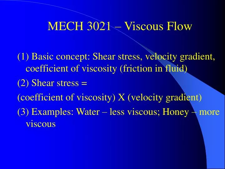
MECH 3021 – Viscous Flow (1) Basic concept: Shear stress, velocity gradient, coefficient of viscosity (friction in fluid) (2) Shear stress = (coefficient of viscosity) X (velocity gradient) (3) Examples: Water – less viscous; Honey – more viscous. Compressible Flows.

E N D
MECH 3021 – Viscous Flow (1) Basic concept: Shear stress, velocity gradient, coefficient of viscosity (friction in fluid) (2) Shear stress = (coefficient of viscosity) X (velocity gradient) (3) Examples: Water – less viscous; Honey – more viscous
Compressible Flows (1) Fluid Mechanics of Flight – Burn fuel to overcome the drag force, or roughly the shear stress at the wall / airplane wing. Hence the dynamics of boundary layer is crucial, i.e. we need to calculate the velocity profile and its derivative: τwis the shear stress divided by viscosity
Compressible Flows (2) The nature of the flow, i.e. laminar (slow, orderly) versus turbulent (fast, chaotic), is critical to this stress, and hence the study of stability is important.
Aerospace (1) Conventional commercial aircrafts typically fly at a Mach number of 0.4 to 0.7. At such speeds, the fluid starts to become compressible. (2) The stability of compressible boundary layers thus deserves serious studies. Given our limitations, we embark on an elementary introduction of compressible flows.
Speed of Sound (1) Signals, information and to some extent energy are transmitted by small disturbances in fluids. Small disturbances in air are known as ‘sound (waves)’. (2) Speed of sound can be computed from a dynamic / thermodynamic consideration. Animation courtesy of Dr. Dan Russell, Kettering University
Reviews of Thermodynamics (1) Adiabatic processes (no heat exchange, temperature will vary) versus Isothermal processes (temperature constant, permit heat exchange). (2) First Law: dQ + dW = dE Heat intothe system work onthe system increase ininternal energy
The Momentum Theorems (1) Linear and angular momentum theorems (2) Control surfaces – conceptual (imaginary) surfaces fixed in space Credit: Cimbala, Cengel (2008), Essentials of Fluid Mechanics: Fundamentals and applications
Volume flow rate = (area)(velocity) Mass flow rate = (density)(area)(velocity) Momentum flow rate = (density)(area)(velocity)2
Linear Momentum theorem :The total external force = rate of change of momentum inside the control surface + the net outflux of momentum from the surface (outflux – influx)
A Heuristic Explanation A typical control volume in a funnel-shaped pipe Fluid contained at t = t0 The fluid at t = t0 + dt Credit: http://www.eng.fsu.edu/~dommelen/courses/flm/rey_tran/index.html
A Heuristic Explanation (Cont’d) To calculate the change of momentum of the fluid considered (Fδt, caused by the external force), the inflow and outflow of the control volume have to be accounted for:
Supersonic, subsonic and transonic flows (1) Flows where the fluid speed exceeds the LOCAL sound speed are known as SUPERSONIC flows. (2) Flows where the fluid speed remains less than the LOCAL sound speed are known as SUBSONIC flows. (3) Flows with both supersonic and subsonic portions are known as TRANSONIC flows.
Basic Gas Laws / Processes (1) Isothermal compression / expansion: (2) Adiabatic compression / expansion:
Sir Isaac Newton (1) Newton invented calculus when he was 23. An epidemic broke out in the UK about three or four hundred years ago. He returned to his rural home and invented calculus in about 18 months. (2) Inspired by an apple falling from a tree, Newton discovered or invented gravitational force.
Sir Isaac Newton (cont’d) (3) Consider the equations of motion in polar coordinates. If the tangential component of the force is zero, while the radial component is an inverse square law in the radius. The solution is an ellipse, and hence he solved the dynamics of the solar system – The Earth moves around the Sun in an elliptical path.
Sir Isaac Newton (cont’d) (4) Newton solved the problem of brachistochrone – minimum time of travel for a falling particle between two points not on the same vertical straight line. (5) BUT, Newton made a mistake in calculating the speed of sound. He used an isothermal, but not the adiabatic, condition. The adiabatic condition is the correct one.
Speed of Sound (1) Speed of sound – change of pressure with respect to density at ADIABATIC conditions. (2) (3) Sound travels FASTER in water than air (and still faster in solids). Contrast this feature with light.
The Energy Equation (1) We first have a ‘reservoir’ of gas at rest (or gas in stagnant condition). (2) The gas is then allowed to flow out from this reservoir through an attached tube / pipe say by a pressure differential (higher pressure in the tank / reservoir). (3) The velocity / kinetic energy acquired must come at the expense of the internal energy, and hence the temperature of the gas MUST DROP as it flows. Reservoir V, ρ P0, T0V=0
Thermodynamic consideration (1) ‘Energy’ of the gas is measured by the enthalpy, or roughly, internal energy + (pressure)(volume). = (roughly CVT + P V) = CV T + RT = (CV + R)T = (specific heat capacity at constant pressure) Multiplied by (temperature)= CpT (2) ‘Energy’ conservation: Enthalpy at reservoir = enthalpy in flow + kinetic energy
Flows through a duct of varying area (1) When a fluid flowing in a pipe / tube encounters a reduction in cross sectional area, our intuition and quantitative studies in incompressible flow earlier tell us that the fluid will speed up. (2) While this remains broadly true for subsonic flows, the statement in point (1) may NOT hold for supersonic flows.
Compressible flows in ducts / pipes / tubes with varying cross sectional areas (1) The law of conservation of mass still holds, which means that the product of (density)(cross sectional area)(velocity) must remain constant. For incompressible fluids, the density is constant and hence our intuition is correct (i.e. area goes down, velocity goes up). (2) For supersonic flows, the density changes drastically with velocity and hence the flow may SLOW down on approaching a reduction in area.
Analysis of flows through a duct of varying area (1) ρV A = constant and hence (2) but from the one dimensional (1D) equations of steady (!!) motion: (3) Speed of sound:
Analysis (continued) (1) (2) M < 1, dA < 0, dV > 0, (3) M > 1, dA < 0, dV < 0 (Counterintuituve!!).
Convergent Nozzles • Subsonic applications Boeing 757 Nozzle Airbus A330 Nozzle Extracted from:http://en.wikipedia.org/wiki/Image:Turbofan_operation.png Extracted from : http://www.astechmfg.com/
Converging-Diverging Nozzles • The nozzle accelerates the flow of a gas from a subsonic to supersonic speed. • In the initial stage, decreasing flow area results in subsonic (M<1) acceleration of the gas. • The area decreases until the “throat” area is reached, where M=1. • Increasing flow area accelerates the flow supersonically (M>1) thereafter. Cimbala and Cengel (2006), Fluid Mechanics: Fundamentals and Applications
Converging-Diverging Nozzles • It is used in rocket engines or other supersonic applications. Photos of a NERVA rocket nozzle on display at the Michigan Space and Science Center (These photos were taken by Richard Kruse in 2002)http://historicspacecraft.com Space Shuttle Main Engine nozzlehttp://www.k-makris.gr/
Shock Waves (1) Generally even the qualitative features of supersonic flows are completely different from those of subsonic flows. (2) Another further distinction is that ‘shock waves’, or surfaces of discontinuities, can occur in supersonic but NOT subsonic flows.
Shock Waves (cont’d) (1) Thought experiment: A gas in a very long cylinder is at rest. A piston is pushed into the gas and the piston is allowed to accelerate. (2) As the gas is compressed, a sequence of wave fronts is generated. However, the wave fronts generated more recently have a higher velocity as the piston is accelerating.
Shock Waves (cont’d) (3) As these ‘younger’ (i.e. generated more recently) wave fronts travel faster than the older wave fronts, we eventually have a piling up of wave fronts, and they form a relatively sharp discontinuity which is known as a shock wave. (4) The thickness of a shock wave is of a few ‘mean free paths’, but in practice the shock is taken as having zero thickness.
Supersonic Flights M=6 M=3.5 Free-flight models of the X-15 being fired into a wind Tunnel vividly detail the shock-wave patterns for airflow. Credit: NASA History Divisionhttp://history.nasa.gov/SP-60/ch-5.html
The Normal Shock Waves (1) A discontinuity of gas properties (in practice, a thin region of rapid changes) perpendicular (normal) to the flow direction. (2) In calculations of textbooks / notes, we go to a frame where the airplane is at rest, and the shock is then stationary ahead of the (supersonic) airplane. In practice, the (supersonic) airplane is flying and the shock is rapidly advancing in a region of much slower moving air (hence the term ‘wave’). slow moving air supersonic air advancingsupersonic airplane at rest advancing shock stationary shock In calculation In practice
The Normal Shock Waves (3) Principles: Conservation of mass, momentum, energy, AND the equation of state make up FOUR equations in four unknowns, velocity, pressure, density and temperature. (4) Conceptually simple but BEWARE of algebra.
Shock waves (continued): (1) Eliminate temperature in the energy equation by the equation of state (2) Use this as the equation for p2 and substitute into the momentum equation. (3) Eliminate ρ2 by the continuity equation to obtain a relation between u2 and u1.
Prandtl’s relation u1u2 = (a*)2 The product of upstream and downstream velocities (relative to the shock) is equal to the square of the sound speed at the place where the flow is sonic.
Rankine Hugoniot Relation This is the relation between the pressure and density ratios across the shock.
Qualitative features of subsonic flows (1) It is possible to hear the sound generated by the aircraft / disturbance from all directions in a sufficiently small neighborhood of the aircraft. (2) A higher frequency is heard in front of the source and a lower frequency is heard behind the source. (Doppler Effect) M = 0.7 Animation courtesy of Dr. Dan Russell, Kettering University
Qualitative features of a sonic flow An observer in front of the source will detect nothing until the source arrives. M = 1 Animation courtesy of Dr. Dan Russell, Kettering University
Qualitative features of supersonic flows Sound waves generated will be confined to within a ‘cone’ (3D) or ‘triangular region’ (2D) of half angle sin–1(1/M) where M is the Mach number. M = 1.4 Animation courtesy of Dr. Dan Russell, Kettering University
Waves and Stabilities in Fluid Flows (1) Stabilities of flows have traditionally been studied by imposing wavy disturbances. (2) For sufficiently small amplitude, the equations of motion are linearized (i.e. linear stability). (3) Physically, interactions among waves are ignored.
Stability (continued) (1) Wave grows – instability; Wave decays – stability General disturbance – superposition, Fourier analysis. (2) Temporal stability – for a fixed wave number or wave length, find the (complex) frequency. Real frequency – neutral or propagating waves. Complex frequency – growing or decaying waves.
Stability (continued) (1) Finite amplitude effects – difficult to impossible to analyze. Numerical or computational approaches. (2) Quasi – parallel flows: e.g. boundary layer, treated as a parallel flow in the leading order approximation.
Dispersive Waves If the (phase) velocity of the wave depends on the wave number (or wave length), the wave is termed dispersive. Implications: a group of waves will ‘disperse’ or ‘disintegrates’ into components in the far field.
Dispersive Waves: Animation • Initial profile is a Gaussian pulse • Black – Non-dispersive wave (maintain a constant shape) • Blue – dispersive wave (“disperse” or “broaden”) Animation courtesy of Dr. Dan Russell, Kettering University
Dispersive Waves (1) The speed / velocity of a wave depends on the wavelength or frequency – Dispersive waves. (2) Examples of NON-dispersive waves – electromagnetic waves in vacuum. (3) Examples of dispersive waves – almost all wave motions in fluids and solids (except sound waves).
Basic terminology on wave motion (1) Meaning of wavelength, frequency, period, velocity (frequency X wavelength) taken as well known. (2) Wave number – number of waves per 2 pi length (or k = 2 pi/wavelength). (3) Angular frequency – 2 pi times frequency. (4) Velocity = (angular frequency)/k
Simple linear partial differential equations as examples (1) Certain simple linear, partial differential equations can be taken as examples for dispersive waves. (2) Relation between angular frequency and wave number – Dispersion Relation.
Dispersion of light in prism (1) Waves with different wavelengths (colors) travel at different speeds. (2) The difference in speed results in different refraction angles (Refractive index = ratio of speeds). (3) Thus, splitting of white light into a rainbow. (Extracted from http://electron9.phys.utk.edu/phys136d/modules/m10/geometrical.htm)
Vorticity (1) Theoretical definition: Curl of the velocity field = . (2) Practical Significance: Twice the local angular velocities. Movie by National Committee for Fluid Mechanics Films (Prof. Ascher Shapiro) Vorticity Meter: From 2:30 to 3:18 Vorticity in straight channel: 3:30 to 3:52 Free vortex: 4:55 to 5:35
Two dimensional ideal incompressible fluid Continuity equation (linear): ux + vy = 0 Equations of motion (nonlinear): ut + uux + vuy = – px /ρ vt + uvx + vvy = – py /ρ