Download
1 / 31
540 likes | 1.23k Views
Combustion Modeling in FLUENT. Outline. Applications Overview of Combustion Modeling Capabilities Chemical Kinetics Gas Phase Combustion Models Discrete Phase Models Pollutant Models Combustion Simulation Guidelines. Temperature in a gas furnace. CO 2 mass fraction. Stream function.

E N D
Outline • Applications • Overview of Combustion Modeling Capabilities • Chemical Kinetics • Gas Phase Combustion Models • Discrete Phase Models • Pollutant Models • Combustion Simulation Guidelines
Temperature in a gas furnace CO2 mass fraction Stream function Applications • Wide range of homogeneous and heterogeneous reacting flows • Furnaces • Boilers • Process heaters • Gas turbines • Rocket engines • Predictions of: • Flow field and mixing characteristics • Temperature field • Species concentrations • Particulates and pollutants
Aspects of Combustion Modeling Combustion Models Dispersed Phase Models Premixed Partially premixed Nonpremixed Droplet/particle dynamics Heterogeneous reaction Devolatilization Evaporation Governing Transport Equations Mass Momentum (turbulence) Energy Chemical Species Radiative Heat Transfer Models Pollutant Models
Combustion Models Available in FLUENT • Gas phase combustion • Generalized finite rate formulation (Magnussen model) • Conserved scalar PDF model (one and two mixture fractions) • Laminar flamelet model (V5) • Zimont model (V5) • Discrete phase model • Turbulent particle dispersion • Stochastic tracking • Particle cloud model (V5) • Pulverized coal and oil spray combustion submodels • Radiation models: DTRM, P-1, Rosseland and Discrete Ordinates (V5) • Turbulence models: k-, RNG k-, RSM, Realizable k- (V5) and LES (V5) • Pollutant models: NOx with reburn chemistry (V5) and soot
Modeling Chemical Kinetics in Combustion • Challenging • Most practical combustion processes are turbulent • Rate expressions are highly nonlinear; turbulence-chemistry interactions are important • Realistic chemical mechanisms have tens of species, hundreds of reactions and stiff kinetics (widely disparate time scales) • Practical approaches • Reduced chemical mechanisms • Finite rate combustion model • Decouple reaction chemistry from turbulent flow and mixing • Mixture fraction approaches • Equilibrium chemistry PDF model • Laminar flamelet • Progress variable • Zimont model
Generalized Finite Rate Model • Chemical reaction process described using global mechanism. • Transport equations for species are solved. • These equations predict local time-averaged mass fraction, mj , of each species. • Source term (production or consumption) for species j is net reaction rate over all k reactions in mechanism: • Rjk (rate of production/consumption of species j in reaction k) is computed to be the smaller of the Arrhenius rate and the mixing or “eddy breakup” rate. • Mixing rate related to eddy lifetime, k /. • Physical meaning is that reaction is limited by the rate at which turbulence can mix species (nonpremixed) and heat (premixed).
Setup of Finite Rate Chemistry Models • Requires: • List of species and their properties • List of reactions and reaction rates • FLUENT V5 provides this info in a mixture material database. • Chemical mechanisms and physical properties for the most common fuels are provided in database. • If you have different chemistry, you can: • Create new mixtures. • Modify properties/reactions of existing mixtures.
Generalized Finite Rate Model: Summary • Advantages: • Applicable to nonpremixed, partially premixed, and premixed combustion • Simple and intuitive • Widely used • Disadvantages: • Unreliable when mixing and kinetic time scales are comparable (requires Da >>1). • No rigorous accounting for turbulence-chemistry interactions • Difficulty in predicting intermediate species and accounting for dissociation effects. • Uncertainty in model constants, especially when applied to multiple reactions.
Conserved Scalar (Mixture Fraction) Approach: The PDF Model • Applies to nonpremixed (diffusion) flames only • Assumes that reaction is mixing-limited • Local chemical equilibrium conditions prevail. • Composition and properties in each cell defined by extent of turbulent mixing of fuel and oxidizer streams. • Reaction mechanism is not explicitly defined by you. • Reacting system treated using chemical equilibrium calculations (prePDF). • Solves transport equations for mixture fraction and its variance, rather than species transport equations. • Rigorous accounting of turbulence-chemistry interactions.
Mixture Fraction Definition • The mixture fraction, f, can be written in terms of elemental mass fractions as: • where Zk is the elemental mass fraction of some element, k. Subscripts F and O denote fuel and oxidizer inlet stream values, respectively. • For simple fuel/oxidizer systems, the mixture fraction represents the fuel mass fraction in a computational cell. • Mixture fraction is a conserved scalar: • Reaction source terms are eliminated from governing transport equations.
Systems That Can be Modeled Using a Single Mixture Fraction • Fuel/air diffusion flame: • Diffusion flame with oxygen-enriched inlets: • System using multiple fuel inlets: 60% CH4 40% CO f = 1 21% O2 79% N2 f = 0 35% O2 65% N2 f = 0 60% CH4 40% CO f = 1 35% O2 65% N2 f = 0 60% CH4 20% CO 10% C3H8 10% CO2 f = 1 f = 0 21% O2 79% N2 60% CH4 20% CO 10% C3H8 10% CO2 f = 1
Equilibrium Approximation of System Chemistry • Chemistry is assumed to be fast enough to achieve equilibrium. • Intermediate species are included.
PDF Modeling of Turbulence-Chemistry Interaction • Fluctuating mixture fraction is completely defined by its probability density function (PDF). • p(V), the PDF, represents fraction of sampling time when variable, V, takes a value between V and V + V. • p(f) can be used to compute time-averaged values of variables that depend on the mixture fraction, f: • Species mole fractions • Temperature, density
PDF Model Flexibility • Nonadiabatic systems: • In real problems, with heat loss or gain, local thermo-chemical state must be related to mixture fraction, f, and enthalpy, h. • Average quantities now evaluated as a function of mixture fraction, enthalpy (normalized heat loss/gain), and the PDF, p(f). • Second conserved scalar: • With second scalar in FLUENT, you can model: • Two fuel streams with different compositions and single oxidizer stream (visa versa) • Nonreacting stream in addition to a fuel and an oxidizer • Co-firing a gaseous fuel with another gaseous, liquid, or coal fuel • Firing single coal with two off-gases (volatiles and char burnout products) tracked separately
Mixture Fraction/PDF Model: Summary • Advantages: • Predicts formation of intermediate species. • Accounts for dissociation effects. • Accounts for coupling between turbulence and chemistry. • Does not require the solution of a large number of species transport equations • Robust and economical • Disadvantages: • System must be near chemical equilibrium locally. • Cannot be used for compressible or non-turbulent flows. • Not applicable to premixed systems.
TheLaminar Flamelet Model • Extension of the mixture fraction PDF model to moderate chemical nonequilibrium • Turbulent flame modeled as an ensemble of stretched laminar, opposed flow diffusion flames • Temperature, density and species (for adiabatic) specified by two parameters, the mixture fraction and scalar dissipation rate • Recall that for the mixture fraction PDF model (adiabatic), thermo-chemical state is function of f only • c can be related to the local rate of strain
Laminar Flamelet Model (2) • Statistical distribution of flamelet ensemble is specified by the PDF P(f,c), which is modeled as Pf (f) Pc(c), with a Beta function for Pf (f) and a Dirac-delta distribution for Pc(c) • Only available for adiabatic systems in V5 • Import strained flame calculations • prePDF or Sandia’s OPPDIF code • Single or multiple flamelets • Single: user specified strain, a • Multiple: strained flamelet library, 0 < a < aextinction • a=0 equilibrium • a= aextinction is the maximum strain rate before flame extinguishes • Possible to model local extinction pockets (e.g. lifted flames)
The Zimont Model for Premixed Combustion • Thermo-chemistry described by a single progress variable, • Mean reaction rate, • Turbulent flame speed, Ut, derived for lean premixed combustion and accounts for • Equivalence ratio of the premixed fuel • Flame front wrinkling and thickening by turbulence • Flame front quenching by turbulent stretching • Differential molecular diffusion • For adiabatic combustion, • The enthalpy equation must be solved for nonadiabatic combustion
Continuous phase flow field calculation Particle trajectory calculation Update continuous phase source terms Discrete Phase Model • Trajectories of particles/droplets/bubbles are computed in a Lagrangian frame. • Exchange (couple) heat, mass, and momentum with Eulerian frame gas phase • Discrete phase volume fraction must < 10% • Although the mass loading can be large • No particle-particle interaction or break up • Turbulent dispersion modeled by • Stochastic tracking • Particle cloud (V5) • Rosin-Rammler or linear size distribution • Particle tracking in unsteady flows (V5) • Model particle separation, spray drying, liquid fuel or coal combustion, etc.
Particle Dispersion: The Stochastic Tracking Model • Turbulent dispersion is modeled by an ensemble of Monte-Carlo realizations (discrete random walks) • Particles convected by the mean velocity plus a random direction turbulent velocity fluctuation • Each trajectory represents a group of particles with the same properties (initial diameter, density etc.) • Turbulent dispersion is important because • Physically realistic (but computationally more expensive) • Enhances stability by smoothing source terms and eliminating local spikes in coupling to the gas phase Coal particle tracks in an industrial boiler
Particle Dispersion: The Particle Cloud Model • Track mean particle trajectory along mean velocity • Assuming a 3D multi-variate Gaussian distribution about this mean track, calculate particle loading within three standard deviations • Rigorously accounts for inertial and drift velocities • A particle cloud is required for each particle type (e.g. initial d,r etc.) • Particles can escape, reflect or trap (release volatiles) at walls • Eliminates (single cloud) or reduces (few clouds) stochastic tracking • Decreased computational expense • Increased stability since distributed source terms in gas phase BUT decreased accuracy since • Gas phase properties (e.g. temperature) are averaged within cloud • Poor prediction of large recirculation zones
Particle Tracking in Unsteady Flows • Each particle advanced in time along with the flow • For coupled flows using implicit time stepping, sub-iterations for the particle tracking are performed within each time step • For non-coupled flows or coupled flows with explicit time stepping, particles are advanced at the end of each time step
Coal/Oil Combustion Models • Coal or oil combustion modeled by changing the modeled particle to • Droplet - for oil combustion • Combusting particle- for coal combustion • Several devolatilization and char burnout models provided. • Note: These models control the rate of evolution of the fuel off-gas from coal/oil particles. Reactions in the gas (continuous) phase are modeled with the PDF or finite rate combustion model.
NOx Models • NOx consists of mostly nitric oxide (NO). • Precursor for smog • Contributes to acid rain • Causes ozone depletion • Three mechanisms included in FLUENT for NOx production: • Thermal NOx - Zeldovich mechanism (oxidation of atmospheric N) • Most significant at high temperatures • Prompt NOx - empirical mechanisms by De Soete, Williams, etc. • Contribution is in general small • Significant at fuel rich zones • Fuel NOx - Empirical mechanisms by De Soete, Williams, etc. • Predominant in coal flames where fuel-bound nitrogen is high and temperature is generally low. • NOx reburn chemistry (V5) • NO can be reduced in fuel rich zones by reaction with hydrocarbons
Soot modeling in FLUENT • Two soot formation models are available: • One-step model (Khan and Greeves) • Single transport equation for soot mass fraction • Two-Step model (Tesner) • Transport equations for radical nuclei and soot mass fraction concentrations • Soot formation modeled by empirical rate constants where, C, pf, and F are a model constant, fuel partial pressure and equivalence ratio, respectively • Soot combustion (destruction) modeled by Magnussen model • Soot affects the radiation absorption • Enable Soot-Radiation option in the Soot panel
Combustion Guidelines and Solution Strategies • Start in 2D • Determine applicability of model physics • Mesh resolution requirements (resolve shear layers) • Solution parameters and convergence settings • Boundary conditions • Combustion is often very sensitive to inlet boundary conditions • Correct velocity and scalar profiles can be critical • Wall heat transfer is challenging to predict; if known, specify wall temperature instead of external convection/radiation BC • Initial conditions • While steady-state solution is independent of the IC, poor IC may cause divergence due to the number and nonlinearity of the transport equations • Cold flow solution, then gas combustion, then particles, then radiation • For strongly swirling flows, increase the swirl gradually
Combustion Guidelines and Solution Strategies (2) • Underrelaxation Factors • The effect of under-relaxation is highly nonlinear • Decrease the diverging residual URF in increments of 0.1 • Underrelax density when using the mixture fraction PDF model (0.5) • Underrelax velocity for high bouyancy flows • Underrelax pressure for high speed flows • Once solution is stable, attempt to increase all URFs to as close to defaults as possible (and at least 0.9 for T, P-1, swirl and species (or mixture fraction statistics)) • Discretization • Start with first order accuracy, then converge with second order to improve accuracy • Second order discretization especially important for tri/tet meshes • Discrete Phase Model - to increase stability, • Increase number of stochastic tracks (or use particle cloud model) • Decrease DPM URF and increase number of gas phase iterations per DPM
Combustion Guidelines and Solution Strategies (3) • Magnussen model • Defaults to finite rate/eddy-dissipation (Arrhenius/Magnussen) • For nonpremixed (diffusion) flames turn off finite rate • Premixed flames require Arrhenius term so that reactants don’t burn prematurely • May require a high temperature initialization/patch • Use temperature dependent Cp’s to reduce unrealistically high temperatures • Mixture fraction PDF model • Model of choice if underlying assumptions are valid • Use adequate numbers of discrete points in look up tables to ensure accurate interpolation (no affect on run-time expense) • Use beta PDF shape
Combustion Guidelines and Solution Strategies (4) • Turbulence • Start with standard k-e model • Switch to RNG k-e , Realizable k-e or RSM to obtain better agreement with data and/or to analyze sensitivity to the turbulence model • Judging Convergence • Residuals should be less than 10-3 except for T, P-1 and species, which should be less than 10-6 • The mass and energy flux reports must balance • Monitor variables of interest (e.g. mean temperature at the outlet) • Ensure contour plots of field variables are smooth, realistic and steady
Concluding Remarks • FLUENT V5 is the code of choice for combustion modeling. • Outstanding set of physical models • Maximum convenience and ease of use • Built-in database of mechanisms and physical properties • Grid flexibility and solution adaption • A wide range of reacting flow applications can be addressed by the combustion models in FLUENT. • Make sure the physical models you are using are appropriate for your application.