Chapter 7 Eigenvalues and Eigenvectors

Chapter 7 Eigenvalues and Eigenvectors 7.1 Eigenvalues and Eigenvectors 7.2 Diagonalization 7.3 Symmetric Matrices and Orthogonal Diagonalization 7.4 Application of Eigenvalues and Eigenvectors 7.5 Principal Component Analysis 7.1

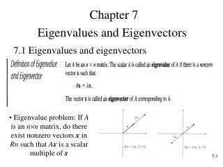
※ Geometric Interpretation Eigenvalue Eigenvector 7.1 Eigenvalues and Eigenvectors • Eigenvalue problem (特徵值問題)(one of the most important problems in the linear algebra): If A is an nn matrix, do there exist nonzero vectors x in Rn such that Ax is a scalar multiple of x？ (The term eigenvalue is from the German word Eigenwert, meaning “proper value”) • Eigenvalue (特徵值)and Eigenvector(特徵向量): A:an nn matrix : a scalar (could be zero) x: a nonzero vector in Rn

Eigenvalue Eigenvalue Eigenvector Eigenvector • Ex 1: Verifying eigenvalues and eigenvectors ※ In fact, for each eigenvalue, it has infinitely many eigenvectors. For  = 2, [3 0]T or [5 0]T are both corresponding eigenvectors. Moreover, ([3 0] + [5 0])T is still an eigenvector. The proof is in Thm. 7.1.

Pf: x1 and x2are eigenvectors corresponding to  • Thm. 7.1: The eigenspace corresponding to  ofmatrix A If A is an nn matrix with an eigenvalue, then the set of all eigenvectors of together with the zero vector is a subspace of Rn. This subspace is called the eigenspace (特徵空間)of  Since this set is closed under vector addition and scalar multiplication, this set is a subspace of Rnaccording to Theorem 4.5

Ex 3: Examples of eigenspaces on the xy-plane For the matrix A as follows, the corresponding eigenvalues are 1 = –1 and 2 = 1: Sol: For the eigenvalue 1 = –1, corresponding vectors are any vectors on the x-axis ※ Thus, the eigenspace corresponding to  = –1 is the x-axis, which is a subspace of R2 For the eigenvalue 2 = 1, corresponding vectors are any vectors on the y-axis ※ Thus, the eigenspace corresponding to  = 1 is the y-axis, which is a subspace of R2

※ Geometrically speaking, multiplying a vector (x, y) in R2by the matrix A corresponds to a reflection to the y-axis

Characteristic polynomial (特徵多項式)of AMnn: • Characteristic equation (特徵方程式)of A: • Thm. 7.2: Finding eigenvalues and eigenvectors of a matrix AMnn Let A be annnmatrix. (1) An eigenvalue of A is a scalar  such that (2) The eigenvectors of A corresponding to  are the nonzero solutions of • Note: follwing the definition of the eigenvalue problem (homogeneous system) has nonzero solutions for x iff (The above iff results comes from the equivalent conditions on Slide 4.101)

Eigenvalue: • Ex 4: Finding eigenvalues and eigenvectors Sol: Characteristic equation:

Ex 5: Finding eigenvalues and eigenvectors Find the eigenvalues and corresponding eigenvectors for the matrix A. What is the dimension of the eigenspace of each eigenvalue? Sol: Characteristic equation: Eigenvalue:

The eigenspace of λ= 2: Thus, the dimension of its eigenspace is 2.

Notes: (1) If an eigenvalue 1 occurs as a multiple root (k times)for the characteristic polynominal, then1 has multiplicity (重數)k. (2) The multiplicity of an eigenvalue is greater than or equal to the dimension of its eigenspace.(In Ex. 5, k is 3 and the dimension of its eigenspace is 2)

Sol: Characteristic equation: Eigenvalues: • Ex 6：Find the eigenvalues of the matrix A and find a basis for each of the corresponding eigenspaces ※ According to the note on the previous slide, the dimension of the eigenspace of λ1 = 1 is at most to be 2 ※ For λ2 = 2 and λ3 = 3, the demensions of their eigenspaces are at most to be 1

is a basis for the eigenspace corresponding to ※The dimension of the eigenspace of λ1 = 1 is 2

Thm. 7.3: Eigenvalues for triangular matrices If A is an nn triangular matrix, then its eigenvalues are the entries on its main diagonal • Ex 7: Finding eigenvalues for triangular and diagonal matrices Sol: ※According to Thm. 3.2, the determinant of a triangular matrix is the product of the entries on the main diagonal

Eigenvalues and eigenvectors of linear transformations: ※ The definition of linear transformation functions should be introduced in Ch 6 ※ Here I briefly introduce the linear transformation and its some basic properties ※ The typical example of a linear transformation function is that each component of the resulting vector is the linear combination of the components in the input vector x • An example for a linear transformation T: R3→R3

Theorem: Standard matrix for a linear transformation

Consider the same linear transformation T(x1, x2, x3) = (x1 + 3x2, 3x1 + x2, –2x3) • Thus, the above linear transformation T is with the following corresponding standard matrix A such that T(x) = Ax ※ The statement on Slide 7.18 is valid because for any linear transformation T:V →V, there is a corresponding square matrix such that T(x) = Ax.Consequently, the eignvalues and eigenvectors of a linear transformation T are in essence the eigenvalues and eigenvectors of the corresponding square matrix A

Transformation matrix for nonstandard bases ※ On the next two slides, an example is provided to verify numerically that this extension is valid

EX. Consider a nonstandard basis to be {v1, v2, v3}= {(1, 1, 0), (1, –1, 0), (0, 0, 1)}, and find the transformation matrix such that corresponding to the same linear transformation T(x1, x2, x3) = (x1 + 3x2, 3x1 + x2, –2x3)

Consider x = (5, –1, 4), and check that corresponding to the linear transformation T(x1, x2, x3) = (x1 + 3x2, 3x1 + x2, –2x3)

Ex 8: Finding eigenvalues and eigenvectors for standard matrices ※ Ais the standard matrix for T(x1, x2, x3) = (x1 + 3x2, 3x1 + x2, –2x3) (see Slides 7.19 and 7.20) Sol:

Notes: The relationship among eigenvalues, eigenvectors, and diagonalization

Keywords in Section 7.1: • eigenvalue problem: 特徵值問題 • eigenvalue: 特徵值 • eigenvector: 特徵向量 • characteristic equation: 特徵方程式 • characteristic polynomial: 特徵多項式 • eigenspace: 特徵空間 • multiplicity: 重數 • linear transformation: 線性轉換

7.2 Diagonalization • Diagonalization problem (對角化問題): For a square matrix A, does there exist an invertible matrix P such thatP–1APis diagonal? • Diagonalizable matrix(可對角化矩陣): Definition 1: A square matrix A is called diagonalizable if there exists an invertible matrix P such thatP–1APis a diagonal matrix (i.e., PdiagonalizesA) Definition 2: A square matrix A is called diagonalizable if A is similar to a diagonal matrix ※ In Sec. 6.4, two square matrices A and B are similar if there exists an invertible matrix P such that B = P–1AP. • Notes: In this section, I will show that the eigenvalue problem is related closely to the diagonalization problem

Pf: • Thm. 7.4: Similar matrices have the same eigenvalues If A and B are similar nn matrices, then they have the same eigenvalues For any diagonal matrix in the form of D = λI, P–1DP = D Consider the characteristic equationof B: Since A and B have the same characteristic equation, they are with the same eigenvalues

Sol: Characteristic equation: • Ex 1: Eigenvalue problems and diagonalization programs

Note: If ※ The above example can verify Thm. 7.4 since the eigenvalues for both A and P–1AP are the same to be 4, –2, and –2 ※ The reason why the matrix P is constructed with the eigenvectors of A is demonstrated in Thm. 7.5 on the next slide

Thm. 7.5: Condition for diagonalization An nn matrix A is diagonalizable if and only if it has n linearly independent eigenvectors ※ If there are n linearly independent eigenvectors, it does not imply that there are n distinct eigenvalues. In an extreme case, it is possible to have only one eigenvalue with the multiplicity n, and there are n linearly independent eigenvectors for this eigenvalue ※ However, if there are n distinct eigenvalues, then there are n linearly independent eivenvectors (see Thm. 7.6), and thus A must be diagonalizable Pf:

Sol: Characteristic equation: • Ex 4: A matrix that is not diagonalizable Since A does not have two linearly independent eigenvectors, A is not diagonalizable.

Step 3: • Steps for diagonalizingan nn square matrix: Step 1: Find n linearly independent eigenvectors for A with corresponding eigenvalues Step 2: Let

Sol: Characteristic equation: • Ex 5: Diagonalizing a matrix

Note: a quick way to calculate Ak based on the diagonalization technique

Thm. 7.6: Sufficient conditions for diagonalization If an nn matrix A has n distinct eigenvalues, then the corresponding eigenvectors are linearly independent and thus A is diagonalizable according to Thm. 7.5. Pf: Let λ1, λ2, …, λn be distinct eigenvalues and corresponding eigenvectors be x1, x2, …, xn. In addition, consider that the first meigenvectors are linearly independent, but the first m+1 eigenvectors are linearly dependent, i.e., where ci’s are not all zero. Multiplying both sides of Eq. (1) by A yields

On the other hand, multiplying both sides of Eq. (1) by λm+1yields Now, subtracting Eq. (2) from Eq. (3) produces Since the first m eigenvectors are linearly independent, we can infer that all coefficients of this equation should be zero, i.e., Because all the eigenvalues are distinct, it follows all ci’s equal to 0, which contradicts our assumption that xm+1 can be expressed as a linear combination of the first m eigenvectors. So, the set of n eigenvectors is linearly independent given n distinct eigenvalues, and according to Thm. 7.5, we can conclude that A is diagonalizable.

Ex 7: Determining whether a matrix is diagonalizable Sol: Because A is a triangular matrix, its eigenvalues are According to Thm. 7.6, because these three values are distinct, A is diagonalizable.

Ex 8: Finding a diagonalized matrix for a linear transformation Sol: The standard matrix for T is given by From Ex. 5 you know that λ1 = 2, λ2 = –2, λ3 = 3 and thus A is diagonalizable. So, according to the result on Slide 7.25, these three linearly independent eigenvectors found in Ex. 5 can be used to form the basis . That is

The matrix for T relative to this basis is ※ Note that it is not necessary to calculate through the above equation. According to the result on Slide 7.25, we already know that is a diagonal matrix and its main diagonal entries are corresponding eigenvalues of A

Keywords in Section 7.2: • diagonalization problem: 對角化問題 • diagonalization: 對角化 • diagonalizable matrix: 可對角化矩陣

Ex 1: Symmetric matrices and nonsymetric matrices 7.3 Symmetric Matrices and Orthogonal Diagonalization • Symmetric matrix (對稱矩陣): A square matrix A is symmetric if it is equal to its transpose: (symmetric) (symmetric) (nonsymmetric)

Thm 7.7: Eigenvalues of symmetric matrices If A is an nn symmetric matrix, then the following properties are true. (1) A is diagonalizable (symmetric matrices are guaranteed to has n linearly independent eigenvectors and thus be diagonalizable). (2) All eigenvalues of A are real numbers. (3) If  is an eigenvalue of A with the multiplicity to be k, then has k linearly independent eigenvectors. That is, the eigenspace of has dimensionk. ※ The above theorem is called the Real Spectral Theorem, and the set of eigenvalues of A is called the spectrum of A.

Pf: Characteristic equation: • Ex 2: Prove that a 2× 2symmetric matrix is diagonalizable. As a function in , this quadratic polynomial function has a nonnegative discriminant (判別式) as follows

The characteristic polynomial of A has two distinct real roots, which implies that A has two distinct real eigenvalues. According to Thm. 7.6, A is diagonalizable.

Thm. 7.8: Properties of orthogonal matrices An nn matrix P is orthogonal if and only if its column vectors form an orthonormal set. • Orthogonal matrix (正交矩陣): A square matrix P is called orthogonal if it is invertible and Pf: Suppose the column vectors of P form an orthonormal set, i.e., It implies that P–1 = PT and thus P is orthogonal.

Chapter 7 Eigenvalues and Eigenvectors