Download
1 / 63
630 likes | 769 Views
Targeting in Multi-Class Screening Under Error and Error Free Measurement Systems. Thesis Defense Presentation on. by ATIQ WALIULLAH SIDDIQUI. PRESENTATION OVERVIEW. Introduction Literature Review Objectives of the Thesis

E N D
Targeting in Multi-Class Screening Under Error and Error Free Measurement Systems Thesis Defense Presentation on by ATIQ WALIULLAH SIDDIQUI
PRESENTATION OVERVIEW • Introduction • Literature Review • Objectives of the Thesis • Multi-Class Screening Model Presented in Min Koo Lee and Joon Soon Jang (1997) • Model Extensions • Sensitivity Analysis • Model Comparisons • Conclusion
WHAT IS QUALITY? • Fitness for Use • Conformance to Specifications • Penalties Associated with Product Deviations Off Target (within specification limits) Customer Tolerance Customer Tolerance Cost of repair, $ Cost of repair, $ LL UL Quality characteristic LL UL Quality characteristic Goal Post Syndrome Taguchi Loss Function
BASIC TARGETING MODEL Model Formulation: Per unit profit function: Per unit Expected profit: Where:
LITERATURE REVIEW C. Springer(1951): The problem was to find the mean for a canning process in order to minimize the cost. The price for producing under/over filled cans are assumed to be different. W. Hunter & C. Kartha (1977): Above problem with under filled item sold in a secondary market. Objective is to maximize of profit. D. Golhar (1987): Under filled cans are to be emptied and refilled at the expense of a fixed reprocessing cost. Cont…
LITERATURE REVIEW M. A. Rahim and P. K. Banerjee (1988): considered the process where the system has a linear drift (e.g., tool wear etc). O. Carlsson (1989): determined, for the case of two variable characteristics, the optimum process mean under acceptance variable sampling. R. Schmidt & P. Pfeifer (1989): investigated the effects on cost savings from variance reduction. K. S. Al-Sultan (1994): addressed the problem of two machines in series. Cont…
LITERATURE REVIEW Liu, Tang and Chun (1995) considered the case of a filling process with limited capacity constraint. F. J. Arcelus (1996) introduced the consistency criteria in the targeting problem. J. Roan, L. Gong & K. Tang (1997) considered production decisions such as production setup and raw material procurement policies. Min Koo Lee & Joon Soon Jang (1997) developed the model for multi-class screening case. Sung Hoon Hong & E. A. Elsayed (1999) studied the effect of measurement error for targeting problem.
OBJECTIVES OF THE THESIS Extend the Min et al. (1997) targeting model for multi class screening incorporating the effects of measurement error. Develop a targeting model for multi class screening incorporating the product uniformity under error free measurement system. Extend the model resulting in objective 2 for the case of measurement systems with error. Study the effects of error in the measurement on the models that will be developed in objective 2 and 3 above
MIN et al. (1997) MODEL Model Assumptions: • A single item is to be sold in two different markets with different cost/profit structures. • The quality characteristic ‘Y’ is assumed normally distributed with unknown process mean and known variance . • The production cost per item is Cont…
Specification limits on ‘Y’ for grade 1 are Specification limits on ‘Y’ for grade 2 are Specification limit s on ‘Y’ for scrap are MIN et al. (1997) Model • Specification limits on different grades are: • 100% inspection is considered
MIN et al. (1997) Model Model Formulation: Per unit profit function: Per unit Expected profit: Where:
OBJECTIVE 1:(Measurement error) Model Assumptions: • A single item is to be sold in two different markets with different cost/profit structures. • The quality characteristic ‘Y’ is assumed normally distributed with unknown process mean and known variance. • The inspection process is error prone. • The measurement ‘X’ is assumed to be unbiased and distributed normally across the true value. • The inspection is based on ‘X’ (observed) as opposed to ‘Y’ (actual) as in Min et al. (1997).
OBJECTIVE 1:(Measurement error) Relationship between ‘X’ and ‘Y’: The ‘X’ is the observed value of ‘Y’ i.e., Where ‘’ is the error in measurement: The expected value of the observed value ‘X’: Cont…
OBJECTIVE 1:(Measurement error) The variance of the observed value ‘X’: The joint distribution of ‘X’ and ‘Y’: or where
OBJECTIVE 1:(Measurement error) Cut off Points: • Instead of the specification limits, inspection is based on ‘Cut off Points’ • Why ‘Cut off Points’? Grade 2 Grade 1 Scrape w2 w1 L2 L1 Targeting with Measurement Error. wi show the ‘Cut off Points’ for the Inspection
OBJECTIVE 1:(Measurement error) Penalties Associated with Misclassifications:
OBJECTIVE 1:(Measurement error) Model Formulation: Per unit profit function: Cont…
OBJECTIVE 1:(Measurement error) Model Formulation: Expected Per unit profit: Where
OBJECTIVE 1:(Measurement error) Sensitivity Analysis: Effect of Error on Expected Profit • 90 problems: • = 0.85, 0.98 ,0.93, 0.97, 0.995 • = 1.25, 1.75 a2-r/a1-a2 = 4, 6, 8 c/a1-a2 = 0.01, 0.15, 0.3 L1 = 41.5, L2 = 40 Cont…
OBJECTIVE 1:(Measurement error) Sensitivity Analysis: Effect of Error on Optimal Mean • 90 problems: • = 0.85, 0.98 ,0.93, 0.97, 0.995 • = 1.25, 1.75 a2-r/a1-a2 = 4, 6, 8 c/a1-a2 = 0.01, 0.15, 0.3 L1 = 41.5, L2 = 40 Cont…
OBJECTIVE 1:(Measurement error) Sensitivity Analysis: Effect of Error on Cut off Points • 90 problems: • = 0.85, 0.98 ,0.93, 0.97, 0.995 • = 1.25, 1.75 a2-r/a1-a2 = 4, 6, 8 c/a1-a2 = 0.01, 0.15, 0.3 L1 = 41.5, L2 = 40 w1 w2 • L1 • L2 Cont…
OBJECTIVE 2:(Uniformity Penalty) Model Assumptions: • A single item is to be sold in two different markets with different cost/profit structures. • The quality characteristic ‘Y’ is assumed normally distributed with unknown process mean and known variance. • The inspection process is error free. • The inspection is based on ‘y’. Cont…
OBJECTIVE 2:(Uniformity Penalty) Model Assumptions: • A quadratic penalty, similar to that of ‘Taguchi Quadratic Loss Function’ is used as a penalty for the item being off target. penalty $ Grade 2 Grade 1 Scrape Target ‘t’ L2 L1 Targeting with Uniformity Penalty ‘t’ shows the Target Value Cont…
OBJECTIVE 2:(Uniformity Penalty) Model Formulation: Per unit profit function: Per unit Expected profit: Where:
OBJECTIVE 2:(Uniformity Penalty) Special Cases: Special case I: (target set at mean) Special case II: (target set at L1)
OBJECTIVE 2:(Uniformity Penalty) Sensitivity Analysis: Effect on Expected Profit • Special Case I • 252 problems: • = 1.5, 1.75, 2, 2.25 a2-r/a1-a2 = 4, 4.5, 5, 5.5, 6, 6.5, 7, 7.5, 8 c/a1-a2 = 0.01, 0.05 0.1, 0.15, 0.2, 0.25, 0.3 L1 = 41.5, L2 = 40 K = 0.05 Cont…
OBJECTIVE 2:(Uniformity Penalty) Sensitivity Analysis: Effect on Optimal Mean • Special Case I • 252 problems: • = 1.5, 1.75, 2, 2.25 a2-r/a1-a2 = 4, 4.5, 5, 5.5, 6, 6.5, 7, 7.5, 8 c/a1-a2 = 0.01, 0.05 0.1, 0.15, 0.2, 0.25, 0.3 L1 = 41.5, L2 = 40 K = 0.05 Cont…
OBJECTIVE 2:(Uniformity Penalty) Sensitivity Analysis: Effect on Expected Profit • Special Case II • 252 problems: • = 1.5, 1.75, 2, 2.25 a2-r/a1-a2 = 4, 4.5, 5, 5.5, 6, 6.5, 7, 7.5, 8 c/a1-a2 = 0.01, 0.05 0.1, 0.15, 0.2, 0.25, 0.3 L1 = 41.5, L2 = 40 K = 0.05 Cont…
OBJECTIVE 2:(Uniformity Penalty) Sensitivity Analysis: Effect on Optimal Mean • Special Case II • 252 problems: • = 1.5, 1.75, 2, 2.25 a2-r/a1-a2 = 4, 4.5, 5, 5.5, 6, 6.5, 7, 7.5, 8 c/a1-a2 = 0.01, 0.05 0.1, 0.15, 0.2, 0.25, 0.3 L1 = 41.5, L2 = 40 K = 0.05 Cont…
OBJECTIVE 3:(Integrated Model) Model Assumptions: • A single item is to be sold in two different markets with different cost/profit structures. • The quality characteristic ‘Y’ is assumed normally distributed with unknown process mean and known variance. • The inspection process is error prone. • The measurement ‘X’ is assumed to be unbiased and distributed normally across the true value. • The inspection is based on ‘X’ (observed) as opposed to ‘Y’ (actual) in last Min et al. (1997). Cont…
OBJECTIVE 3:(Integrated Model) Model Assumptions: • A quadratic penalty, similar to that of ‘Taguchi Quadratic Loss Function’ is used as a penalty for the item being off target. penalty $ Grade 2 Grade 1 Scrape Target ‘t’ w2 w1 L2 L1 Targeting with Measurement Error & Uniformity Penalty ‘t’ shows the Target Value & wi represent the Cut off Points
OBJECTIVE 3:(Integrated Model) Relationship between ‘X’ and ‘Y’: The ‘X’ is the observed value of ‘Y’ and the joint distribution is: or Cut off Points: • Instead of the specification limits, inspection is based on ‘Cut off Points’ • Why ‘Cut off Points’?
OBJECTIVE 3:(Integrated Model) Penalties for misclassification:
OBJECTIVE 3:(Integrated Model) Model Formulation: Per unit profit function:
OBJECTIVE 3:(Integrated Model) Model Formulation: Expected Per unit profit: Where
OBJECTIVE 3:(Integrated Model) Special Cases: Special case I: (target set at mean) Special case II: (target set at L1)
OBJECTIVE 3 :(Integrated Model) Sensitivity Analysis: Effect on Expected Profit • Special Case I • 90 problems: • = 0.85, 0.98 ,0.93, 0.97, 0.995 • = 1.25, 1.75 a2-r/a1-a2 = 4, 6, 8 c/a1-a2 = 0.01, 0.15, 0.3 L1 = 41.5, L2 = 40 K = 0.05 Cont…
OBJECTIVE 3 :(Integrated Model) Sensitivity Analysis: Effect on Optimal Mean • Special Case I • 90 problems: • = 0.85, 0.98 ,0.93, 0.97, 0.995 • = 1.25, 1.75 a2-r/a1-a2 = 4, 6, 8 c/a1-a2 = 0.01, 0.15, 0.3 L1 = 41.5, L2 = 40 K = 0.05 Cont…
OBJECTIVE 3 :(Integrated Model) Sensitivity Analysis: Effect on Cut off Points • Special Case I • 90 problems: • = 0.85, 0.98 ,0.93, 0.97, 0.995 • = 1.25, 1.75 a2-r/a1-a2 = 4, 6, 8 c/a1-a2 = 0.01, 0.15, 0.3 L1 = 41.5, L2 = 40 K = 0.05 w1 w2 • L1 • L2 Cont…
OBJECTIVE 3 :(Integrated Model) Sensitivity Analysis: Effect on Expected Profit • Special Case II • 90 problems: • = 0.85, 0.98 ,0.93, 0.97, 0.995 • = 1.25, 1.75 a2-r/a1-a2 = 4, 6, 8 c/a1-a2 = 0.01, 0.15, 0.3 L1 = 41.5, L2 = 40 K = 0.05 Cont…
OBJECTIVE 3 :(Integrated Model) Sensitivity Analysis: Effect on Optimal Mean • Special Case II • 90 problems: • = 0.85, 0.98 ,0.93, 0.97, 0.995 • = 1.25, 1.75 a2-r/a1-a2 = 4, 6, 8 c/a1-a2 = 0.01, 0.15, 0.3 L1 = 41.5, L2 = 40 K = 0.05 Cont…
OBJECTIVE 3 :(Integrated Model) Sensitivity Analysis: Effect on Cut off Points • Special Case II • 90 problems: • = 0.85, 0.98 ,0.93, 0.97, 0.995 • = 1.25, 1.75 a2-r/a1-a2 = 4, 6, 8 c/a1-a2 = 0.01, 0.15, 0.3 L1 = 41.5, L2 = 40 K = 0.05 w1 w2 • L1 • L2 Cont…
MODEL COMPARISON Numerical Comparison: % Gain in Profit • EMP1 vs. EMP2 • 90 problems: • = 0.85, 0.98 ,0.93, 0.97, 0.995 • = 1.25, 1.75 a2-r/a1-a2 = 4, 6, 8 c/a1-a2 = 0.01, 0.15, 0.3 L1 = 41.5, L2 = 40
MODEL COMPARISON Analytic Comparison: • To show that some models are special cases of the others EPM1 vs. EPM2: • It is clear that as • Also, • Since it was assumed that i.e., it is clear that
MODEL COMPARISON • Since, , & at , it can be shown that: • Also by using L’hospital rule it can be shown that the penalty terms containing the bivariate normal distribution will vanish at
MODEL COMPARISON • Therefore at the relationship for EPM2 i.e., can be written as: • EMP2 EMP1 as
MODEL COMPARISON Analytic comparison: EPM1 vs. EPM3: • At K = 0 • EMP3 EMP1 as