Download
1 / 26
260 likes | 267 Views
Haplotype Phasing using Semidefinite Programming. Parag Namjoshi CSEE Department University of Maryland Baltimore County. Joint work with Konstantinos Kalpakis. Outline. Biology Review Motivation Previous work Our contribution Experimental results Conclusions. Biology Review.

E N D
Haplotype Phasing using Semidefinite Programming Parag Namjoshi CSEE Department University of Maryland Baltimore County Joint work with Konstantinos Kalpakis BIBE 05
Outline • Biology Review • Motivation • Previous work • Our contribution • Experimental results • Conclusions BIBE 05
Biology Review • living systems are composed of cells • the code for the creation of the cells is packed in a molecule called DNA. • DNA consists of four nucleic acids Adenine, Cytosine, Guanine, and Thymine arranged as complementary strands of a double helix. • DNA strand = string of A,C,G, & T’s. BIBE 05
Chromosomes • the genome is arranged as set of distinct chromosomes. • mammals are diploids • humans have 22 + x and y chromosomes. • chromosomes occur in homologous pairs • one homologous chromosome is inherited from each parent • homologous chromosomes contain the same genes in the same order (up to mutations) BIBE 05
Single Nucleotide Polymorphisms. • Single Nucleotide Polymorphism (SNP) = mutation of a single base. • evidence suggests that in humans • 90% of variation is due to SNPs • DNA has long conserved regions punctuated by SNPs • there is one SNP in approximately 1000 bases • most SNPS are bi-allelic • at any given locus, only two of the four possible nucleotides are present in 95% of the population • the restriction (projection) of a DNA strand to SNP sites is a haplotype BIBE 05
What are Genotypes? • the genotype of diploid organisms is the conflation of the inherited haplotypes BIBE 05
Genotype & Haplotype Std. Representation • genotypes and haplotypes can be represented as a 0,1,2 vectors • independently for each site • identify each one of the two letters that appear in it with 0 or 1 • replace each homozygous site with 0/1 using the mapping above • replace heterozygous sites with 2 BIBE 05
Haplotypes vs. Genotypes • large scale polymorphism studies such as Linkage Disequilibrium need haplotype information • however, experimentally • it is expensive to segregate the haplotypes of the individuals • it is easier to observe the genotypes of those individuals • can we find haplotypes from the genotypes computationally? • a genotype with h heterozygous sites can be explained (phased) by 2h-1 different haplotype pairs • how do you choose among them? BIBE 05
Haplotype Phasing with Parsimony • in Population haplotyping, given genotypes from different individuals we want to find a set of haplotypes which resolve all the genotypes • Recall that there can be many such solutions • Experimental evidence suggests that the number of such haplotypes is small • HPP: Haplotype Phasing Problem with Pure Parsimony • Given a set of genotypes, find a minimum size set of haplotypes which conflate to produce the given genotypes • other criteria for choosing among possible sets of haplotypes are • perfect phylogeny, minimum total pairwise distance, minimum diameter, etc • we focus on HPP problem • Lancia, Pinotti, and Rizzi proved that the HPP is NP–complete as well as APX–hard BIBE 05
Clark’s Rule • Clark (1990) describes a greedy inference rule to find a small set of haplotypes resolving a set of genotypes • Starting with a set of haplotypes H that resolves all the homozygous genotypes, do the following • for each unresolved genotype g • if there is a pair (h, h’) that resolves g with h in H, then add h’ to H, else stop • the solution obtained is sensitive to the order in which genotypes are resolved • Clark’s rule may terminate with some genotypes unresolved (orphans) • The rule can be modified to include a pair of haplotypes that resolve an orphan genotype, and continue as before BIBE 05
Gusfield’s TIP • Gusfield (1999) introduces the TIP approach • enumerate all distinct haplotypes that can be used to resolve any single heterozygous genotype • solve an Integer linear Program (IP) to select a minimum size set haplotypes from the enumerated haplotypes that explains the genotypes • TIP uses O(2L n) variables and constraints, where L is the maximum number of heterozygous loci of any genotype • Gusfield describes a number of important improvements to the basic approach above that improve performance BIBE 05
Harrower-Brown IP • Harrower and Brown give an alternate 0-1 IP for the HPP problem (HB-IP) • explain the n genotypes with 2n haplotypes (not necessarily distinct) • the number of distinct haplotypes used are minimized • the number of variables and constraints is polynomial in n, m BIBE 05
The QIP approach - Outline • arithmetic representation of genotypes • semidefinite programming (SDP) • Quadratic Integer Program (QIP) for HPP • a semidefinite programming based heuristic to solve QIP • experimental results • concluding remarks BIBE 05
Arithmetic Representation of Genotypes • represent each genotype g as a vector δ with • each homozygous locus takes value 0 or 2 iff it was 0 or 1 in g • each heterozygous locus takes value 1 • conflation can now be replaced by addition • if haplotypes h1 andh2 explain genotype δ, then • δ = h1 + h2 • we call δ an arithmetic genotype g = 0 1 2 h1= 0 1 0 h2= 0 1 1 δ = 0 2 1 h1= 0 1 0 h2= 0 1 1 g δ BIBE 05
Arithmetic Genotypes • let Δ be n x m matrix with the arithmetic genotypes as rows • let H be k x m matrix with haplotypes as rows • if haplotypes in H resolve Δ, then Δ = S H • where S is a n x k 0-1-2 matrix • the row of S for a homozygous genotype has a single 2 • all other rows have exactly two 1s • we call S a selector matrix • ith row of S “selects” two haplotypes (rows of H) to explain ith genotype BIBE 05
The k-HPP Problem • the k-HPP problem • Given nxm matrix Δ representing a set of n distinct genotypes each with m loci • Find an nxk 0-1-2 selector matrix S and a kxm 0-1 haplotype matrix H such that • Δ = S H • S has as few non-zero columns as possible • all row-sums of S are 2 • HPP is equivalent to k-HPP with k=2n • lower Bounds for HPP • is a well known lower bound • Lemma: rank(Δ) is a lower bound for HPP • Consider an optimal solution S, H • Since Δ = S H, we know that rank(Δ) = min(rank(S), rank(H)), and thus H must have at least rank(Δ) distinct rows (haplotypes) BIBE 05
Finding H given Δ and S • given Δ and H to find an S is easy • given Δ and S find an H by solving a 2-SAT problem • If genotype i is resolved by haplotypes t and l, then for each locus j, add following clauses • If δi,j = 0, add two clauses (¬ht,j)^ (¬hl,j) • If δi,j = 2, add two clauses (ht,j)^ (hl,j) • If δi,j = 1, add clauses (ht,j V hl,j ) ^ (¬ht,j V ¬hl,j) • Only one of the ht,j ,hl,j must both be 1 • 2-SAT problem • has km variables and 2nm clauses • can be solved in (almost) linear time • any satisfying assignment gives a resolution of the genotypes BIBE 05
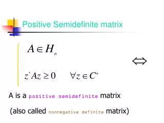
Quadratic, Vector, and Semi-definite Programs • Quadratic Integer Program • Optimize a quadratic objective function subject to quadratic constraints on integer variables • Strict, when each term has total degree 0 or 2 • Vector program • optimize a linear objective function of inner products of vector variables subject to linear constraints on inner products of those variables • Strict quadratic programs lead to vector programs (products of variables are mapped to inner products of corresponding vectors) • SDP program • optimize a linear objective function of the elements of a matrix X subject to • linear constraints on the elements of X • X being a positive semi-definite matrix • Vector programs lead to SDP (X is the matrix of all vector inner products) • SDP programs can be solved in polynomial-time with small numerical errors, thus • solving vector programs, thus • solving relaxations of strict Quadratic Integer programs • construct an approximate solution to a quadratic integer program from a solution of its relaxation, obtained via SDP BIBE 05
Quadratic Integer Program for the k-HPP Subject to: BIBE 05
QIP Heuristic: SDP+Rounding+Backtracking • recursively solve k-HPP • using SDP compute vectors for the variables of QIP • for each selector variable Si,j, compute • P[Si,j]=probability that a random hyperplane separates the vectors of Si,j and z variables (ala MAX-CUT) • round to 1 the Si,j* with the highest P[Si,j] • residual k-HPP=k-HPP problem with the rounded Si,j’s fixed to their rounded value • if the residual k-HPP is infeasible • round Si,j* to 0 instead • if the new residual k-HPP is still infeasible • backtrack by returning infeasible • recursively solve the residual k-HPP BIBE 05
Experiments • we experiment with three approaches for the HPP problem • Clark’s rule • LP relaxation of Gusfield’s TIP scheme with simple rounding • the QIP heuristic for k–HPP with k = 2n • The MATLAB package SDPT 3.02 is used to solve the SDP relaxation of the problem • all experiments are done on a single CPU MATLAB on a Dual Xeon 2.4 Ghz desktop with 1GB memory BIBE 05
Experimental Datasets • we use synthetic datasets A and B • each with 20 instances for each triplet (n, m, k) = (5, 5, 5), (8, 8, 8), (10, 10, 10), and (15, 15, 15) (and for B, recombination levels ρ = 0, 16 and 40) • generate instances of the HPP problem as follows • randomly mate k haplotypes with m loci to produce n genotypes • generation of haplotypes for dataset A • each locus of k haplotypes takes value 0/1 with probability ½ independent of other loci and other genotypes • generation of haplotypes for dataset B • Use Hudson’s program to generate haplotypes with these parameters • diploid population of size 106 • mutation rate = 1.5 × 10⁻⁶ • recombination levels ρ = 0, 16 and 40 corresponding to crossover probabilities 0, 4 × 10⁻⁶, and 10-5 BIBE 05
Experimental Results BIBE 05
QIP Extensions • QIP can be extended to handle many variants of basic k-HPP problem, such as • partial Genotypes • Some loci in some genotypes are unknown • shared haplotypes • Prior knowledge of shared haplotypes • allowing for erroneous genotypes and loci editing • allowing for outlier genotypes BIBE 05
Concluding Remarks • developed arithmetic formulation for the HPP problem • provides new lower bound • yields simple quadratic IP (QIP) • QIP can be extended to handle many variants, incorporate prior information etc • SDP relaxation of QIP that can be solved in polynomial time • SDP+rounding+backtracking gives QIP heuristic • experimentally • Demonstrate competitiveness of QIP heuristic vs Clark’s rule and Gusfield’s TIP relaxation • Show that rank of the genotypes is a tighter lower bound than • future work • Analysis of worst-case performance ratio of the QIP heuristic • Devise algorithms that scale better BIBE 05
Thank You ! Questions ? BIBE 05