Download

1 / 27
480 likes | 1.07k Views
Reliability Prediction. By Yair Shai. A Quest for Reliable Parameters. Goals. Compare the MTBCF & MTTCF parameters in view of complex systems engineering. Failure repair policy as the backbone for realistic MTBCF calculation.

E N D
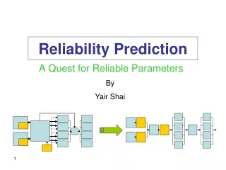
Reliability Prediction By Yair Shai A Quest for Reliable Parameters
Goals • Compare the MTBCF & MTTCF parameters in view of complex systems engineering. • Failure repair policy as the backbone for realistic MTBCF calculation. • Motivation for modification of the technical specification requirements.
Promo : Description of Parameters t1 t2 t3 t4 t5 ....... time r =Number ofFailures Failure Event of an Item Repairable Items: Mean Time Between Failures = Semantics ? Non Repairable Items: Mean Time To Failure =
MTBF = MTTF ?? An assumption: Faileditem returns to “As Good As New” status after repair or renewal. note: Time To Repair is not considered. UP TIME DOWN
Critical FailuresMoving towards System Design A System Failure resulting in (temporary or permanent) Mission Termination. X COMPUTER A simple configuration of parallel hot Redundancy. SUBSYSTEM X COMPUTER A Failure: any computer failure A Critical Failure: two computers failed
Critical Failures A clue for Design Architecture MTBCF Mean Time Between Critical Failures MTTCF Mean Time To Critical Failure SAME? Remember the assumptions Determining the failure repair policy: COLD REPAIR No time for repair actions during the mission
Functional System Design Switch control UNIT A ANTENA CPU 4 CHANNEL RECEVER CONTROLER POWER SUPPLY UNIT B ANTENA sw UNIT C ANTENA CPU POWER SUPPLY UNIT D ANTENA POWER SUPPLY 2 / 4 Operational Demand: At least two receiver units and one antenna should work to operate the system.
From System Design to Reliability Model A ANT CPU PS1 INDEPENDENT BLOCKS B ANT CONT PS2 sw x C ANT CPU PS1 x x D ANT Is this a Critical Failure ? 2 / 4 Serial model : Rs = R1x R2 Parallel model : Rs = 1- (1-R1)x(1-R2) K out of N model : Rs = Binomial Solution
From RBD Logic Diagram to Reliability Function Simple mathematical manipulation: Rsys(t)= f( serial / parallel / K out of N) Classic parameter evaluation: WARNING !!! Is this realistic ? MTTCF MTBCF After each repair of a critical failure- The whole system returns to status “As Good As New”. [ S.Zacks, Springer-Verlag 1991, Introduction To Reliability Analysis, Par 3.5]
MTBCF vs. MTTCFA New Interpretation First Common practice interpretation: MTBCF = MTTCF = MTTCFF Each repair “Resets” the time count to idle status (or) Each failure is the first failure. Realistic interpretation: MTBCF = MTTCF Only failed Items which cause the failure are repaired to idle. All other components keep on aging.
PresentationI Simple 3 aging components serial system model HAD WE KNOWN THE FUTURE… A B C A 3 2 1 2 B 2 2 3 1 3 C 3 2 1 1 1 TTCF
PresentationII Simple 3 aging components serial system model HAD WE KNOWN THE FUTURE… A B C A 4 3 2 1 B 2 1 3 C 1 2 3 4 TBCF
Presentation III Simple 3 aging components serial system model HAD WE KNOWN THE FUTURE… A B C A 4 3 2 1 B 2 1 3 C 1 2 3 4 TBCF MTBCF < MTTCF A 3 2 1 2 B 2 2 3 1 3 C 3 2 1 1 1 TTCF
Simulation Method MONTE – CARLO MATHCAD MIN (X1,1 X2,1 X3,1) MIN (X1,1 X2,1 X3,1) MIN (X1,2 X2,2 X3,2) MIN (X1,2 Δ1,2Δ2,2) N=100,000 SETS N=100,000 SETS ……………………. ……………………. MIN (X1,N X2,N X3,N) MIN (X1,N Δ1,NΔ2,N) _________________ _________________
How “BIG” is the Difference ? 1. Depends on the System Architecture. 2. Depends on the Time-To-Failure distribution of each component. 3. The difference in a specific complex electronic system was found to be ~40% Note: True in redundant systems even when all components have constant failure rates.
Why Does It Matter ? Suppose a specification demand for a system’s reliability : MTBCF = 600 hour Suppose the manufacturer prediction of the parameter: MTBCF = 780 hour -40% X ATTENTION !!! How was it CALCULATED ???? Is this MTBCF or MTTCF ???? “Real” MTBCF = 480 < 600 (spec)
Example 1 Aging serial system – each component is weibull distributed
Example 2 Two redundant subsystems in series – each component is exponentially distributed
serial Constant failure rate parallel
A Comment about Asymptotic Availability (*) (*) [ S.Zacks, Springer-Verlag 1991, Introduction To Reliability Analysis, Par 4.3]
Repair policies • “Hot repair” is allowed for redundant components. • All components are renewed on every failure event. • All failed components are renewed on every failure event. • Failed components are renewed only in blocks which caused the system failure. • Failed subsystems are only partially renewed.
Conclusions • System configuration and distribution of components determine the gap. • Repair policy should be specified in advance to determine calculation method. • Flexible software solutions are needed to simulate real MTBCF for a given RBD. • Predict MTBCF not MTTCF