Download
1 / 17
190 likes | 404 Views
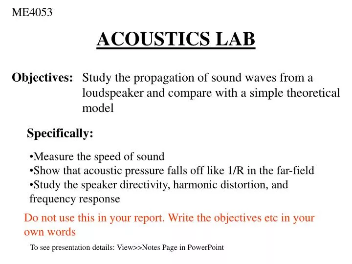
ACOUSTICS LAB. ME4053. Objectives: Study the propagation of sound waves from a loudspeaker and compare with a simple theoretical model. Specifically:. Measure the speed of sound Show that acoustic pressure falls off like 1/R in the far-field

E N D
ACOUSTICS LAB ME4053 Objectives: Study the propagation of sound waves from a loudspeaker and compare with a simple theoretical model Specifically: • Measure the speed of sound • Show that acoustic pressure falls off like 1/R in the far-field • Study the speaker directivity, harmonic distortion, and frequency response Do not use this in your report. Write the objectives etc in your own words To see presentation details: View>>Notes Page in PowerPoint
Experimental Procedure for: • Speed of sound measurement • 1/R acoustic pressure behavior in far-field Note: signal parameter values vary from A-sections to B-sections and from semester to semester. Refer to “Procedures” document for numerical values • Keep the speaker fixed • Vary the mic distance, R • Record time delay • Record rms voltage
Experimental Procedure for Capturing Sample a Waveform Save waveforms to Floppy Drive: • Move mic a distanceR_w from baffle • Save input waveform • Save output waveform • See later slide for processing
Experimental Procedure for Harmonic Distortion and Frequency Response • Obtain Harmonic Distorion: • Fix mic at distance R_df • Use Oscilloscope Math FFT • Record amplitude at a “loud” volume • Decrease volume until main peak is 12dB lower • Record magnitude of second peak • Obtain Frequency Response: • Record the RMS voltage of the microphone over a set of frequencies at two different speaker angles.
Experimental Procedure (cont’d) • Get your notebook signed • Turn all equipment off (especially the mic!) • Leave the lab (you don’t have to go home but you can’t stay here)
T T Time Delay & RMS Voltage Measurements @ = xx s ∆ = xx s Ch 2 = xx V RMS Ch 1 Input Gating ON gives RMS value only between two cursors Ch 2 Output @ ∆ ∆ should remain constant as it is simply the period of the burst @ gives distance from trigger to solid cursor. This is an easy way to measure time delay.
Post-Lab Data Analysis for Sound Pressure Level • Calculate sound pressure level (SPL) in terms of decibels (dB) • Plot the SPL as a function of log(R/Rmin) • Verify that the SPL approaches a -20 dB/decade slope sufficiently far from the speaker
Sound Pressure Level (SPL) Decay SPL decay approaches 1/R (-20dB per decade) model in far field (students may look different)
Post-Lab Data Analysis forSpeed of Sound Plot the data: • Perform a regression on the data • Be sure you have at least 4 significant digits in the slope estimate • Calculate theoretical value of speed of sound • Estimate the “standard error” in your result using the formulas on the next slide • You may want to use Matlab’s “regress” function or Excel’s “linest” function to calculate s est • Compare theoretical and experimental values
Error Analysis Standard Error of the tarr Estimate Standard Error of the Slowness (Slope) Estimate Data Arrival Time (m sec) Range(m)
Post-Lab Data Analysis for Captured Waveform • Compare input and output signal • Plot .input and output signals using Matlab. The “subplot” command is useful for this • Discuss the differences between waveforms • Note: t=0 on the abscissa is the trigger point for input signal • (The results shown below are for a 5 kHz 10 cycle signal )
Post-Lab Analysis for Frequency Response and Harmonic Distortion • Plot the Frequency Response for both the directly facing and 70 degree speaker data. • Convert the voltages to dB using: 20*log10(voltage) • Use directivity theory: Theoretical 70 degree response is equal to 20*log10(voltages@0 degrees) – absolute(20*log10(D(theta))) see future slide for D(theta) and plot. • Then plot in Matlab: semilogx(frequencies, dBvalues) • Take an average dB over 150-12800 Hz and calculate the distance to the largest outlier in that rage. • Harmonic Distortion calculate the dB ratios, is the speaker more pure at lower volumes?
Frequency Response Example Plot Based on this plot can you tell if higher or lower frequencies are more directive and does this speaker provide a flat response over this frequency range?
Post-Lab Data Analysis Directivity Help • Theoretical directivity pattern • Where: k is the wave number, a is the radius of the source, and J1 is a bessel function of the first order. • At low frequencies (where l > a), the function D(q) does not exhibit many variations as a function of q ==> speaker is weakly directional • At higher frequencies (when l < a), D is more dependent on the values of q ==> the speaker is highly directional
Sample code to read comma delimited text file in Matlab %This file will read a comma delimited file %generated from the Tektronix Oscilloscope %It will then plot the data % %Created by: Wayne M. Johnson 17MAR03 % clear all; %clears all variables close all; %closes all figure windows a=dlmread('TEK00000.CSV'); %reading comma delimited file tin=a(:,1)*1e3; %assigning the time data %Note that time data has been shifted to such that %t=0 corresponds to the trigger point for input signal. % See Tektronix User Manual, p. 3-47 Vin=a(:,2); %assigning the voltage data a=dlmread('TEK00001.CSV'); %reading comma delimited file tout=a(:,1)*1e3; %assigning the time data Vout=a(:,2); %assigning the voltage data %plotting data subplot(2,1,1); plot(tin,Vin);grid %plotting the data title('Input signal XXX kHz');ylabel('Voltage (V)'); subplot(2,1,2); plot(tout,Vout);grid %plotting the data title('Microphone output at YYY cm from speaker'); xlabel('Time (msec)');ylabel('Voltage (V)');
Last minute pointers • Your presentations should be much better than this one. Use your own words! • For help contact the TA’s • See Class syllabus for Dates/Times of Presentations and Abstract Submission • Both submissions will be done with your group