The Latent Maximum Entropy Principle for Language Modeling

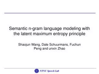
1. The Latent Maximum Entropy Principle for Language Modeling Hsuan-Sheng Chiu Reference: Rosenfeld, “A Maximum Entropy Approach to Adaptive Statistical Language Modeling, 1996 Chen, et al. “A Survey of Smoothing Techniques for ME Models”, 2000 Wang, et al. “The Latent Maximum Entropy Principle”, 2003 Wang, et al. “Combining Statistical Language Models via Latent Maximum Entropy Principle, 2005

2. Outline • Introduction • ME • LME • Conclusion

3. History of Maximum Entropy • Ed. T. Jaynes, “Information Theory and Statistical Mechanics”, 1957 • “Information theory provides a constructive criterion for setting up probability distributions on the basis of partial knowledge, and leads to a type of statistical inference which is called the maximum entropy estimate. It is least biased estimate possible on the given information; i.e., it is maximally noncommittal with regard to missing information”. • http://bayes.wustl.edu/etj/etj.html • Stephen A. Della Pietra and Vincent J. Della Pietra, “Statistical Modeling by Maximum Entropy”, 1993 • Fuzzy ME • Adam L. Berger, Stephen A. Della Pietra and Vincent J. Della Pietra, “A Maximum Entropy Approach to Natural Language Processing”,1996 • First introduced to NLP (LM) • Ronald Rosenfeld, “A Maximum Entropy Approach to Adaptive Statistical Language Modeling”, 1996

4. History of Maximum Entropy (cont.) • Shaojun Wang, Ronald Rosenfeld and Yunxin Zhao, “Latent Maximum Entropy Principle For Statistical Language Modeling” ,ASRU 2001 • LME principle • Other papers about ME: • R. Rosenfeld et al. “Whole-sentence exponential language models: a vehicle for linguistic-statistical integration”, 2001 • S. Wang et al. “Semantic n-gram Language Modeling with the Latent Maximum Entropy Principle”, ICASSP 2003 • C-H. Chueh et al. “A maximum Entropy Approach for Integrating Semantic Information in Statistical Language Models”, ISCSLP 2004 • C-H. Chueh et al. “Discriminative Maximum Entropy Language Model for Speech Recognition”, Interspeech 2005 • C-H. Chueh et al. “Maximum Entropy Modeling of Acoustic and Linguistic Features”, ICASSP 2006

5. Introduction • The quality of a language model M can be judged by its cross entropy with the distribution of some hitherto unseen text T • The goal of statistical language modeling is to identify and exploit sources of information in the language stream, so as to bring the cross entropy down, as close as possible to the true entropy

6. Introduction (cont.) • Information Sources (in the Document’s History) • Context-free estimation (unigram) • Short-term history (n-gram) • Short-term class history (class n-gram) • Intermediate distance (skip n-gram) • Long distance (trigger) • (Observed information) • Syntactic constraints

7. Introduction (cont.) • Combining information sources • Linear interpolation • Extremely general • Easy to implement, experiment with and analyze • Can not hurt (no worse than any of its components) • Suboptimal ? • Inconsistent with components • Backoff

8. The Maximum Entropy Principle • Under the Maximum Entropy approach, one does not construct separate models. Instead, one builds a single, combined model, which attempts to capture all the information form various knowledge source. • Constrained optimization • a) all p are allowable • b) p lying on the line are allowable • c) p at intersection are allowable • d) no model can satisfy

9. The Maximum Entropy Principle (cont.) • Estimate • The bigram assigns the same probability estimate to all events in that class • Mutually inconsistent. How to reconcile? • Linear interpolation • Backoff • ME

10. The Maximum Entropy Principle (cont.) • ME does away with the inconsistency by relaxing the conditions imposed by the component sources • Only requires probability P be equal to K on average in the training data • There are many different function P that would satisfy it • Try to find out the model p among all the function in that intersection that has the highest entropy

11. The Maximum Entropy Principle (cont.) • Information Sources as Constraint Functions • Index function (selector function) • So • Any real-valued function can be used. • Constraint function

12. The Maximum Entropy Principle (cont.) • Constrained optimization (primal) • Lagrangian

13. Derivation of Exponential Form

14. Exponential Form • Exponential form • Dual function • Suppose that λ* of Ψ(λ) is the solution of the dual problem, then p λ* is the solution of the primal problem • The maximum entropy model subject to the constraints hasp parametric form p λ*, where the parameter values λ* can be determined by maximizing the dual function Ψ(λ)

15. Duality • Robert M. Freund, “Applied Lagrange Duality for Constrained Optimization”, 2004

16. Duality (cont.)

17. Relation to Maximum Likelihood • Definition of log-likelihood • Replace p with exponential form • Dual function equals to log-likelihood of the training data • The model with maximum entropy is the model in the parametric family that maximizes the likelihood of the training data

18. Improved Iterative Scaling (IIS) • IIS performs hill-climbing in the log-likelihood space with enforcement of two relax lower bounds • Adam Berger, “The Improved Iterative Scaling Algorithm: A Gentle Introduction”, 1997 • Rong Yan, “A variant of IIS algorithm” • Definition of difference of likelihood function

19. Improved Iterative Scaling (IIS) (cont.) • derivation

20. Improved Iterative Scaling (IIS) (cont.)

21. Improved Iterative Scaling (IIS) (cont.) Jensen Inequality：

22. Improved Iterative Scaling (IIS) (cont.) • It is straightforward to solve for each of the n free parameters individually by differentiating with respect to δ in turn • In case f#(h,w) is constant for each (h,w) pair, IIS can be degraded to the GIS algorithm and simply solved in close-form • Otherwise, this can solve with numeric root-finding procedure

23. IIS (cont.) • Input: feature function ; empircal distribution • Output: Optimal parameter values ; optimal model • 1. start with for all • 2. do for each • Let be the solution to where b. Update the value of according to: • 3. Go to step 2 if not all the have converged

24. IIS (cont.) • Assume , considered trigram model only • For each pair (h,w) , may be 3,2,or 1 • We can arrange the coefficient of x by the order are model probabilities of one pair (h,w) is empirical distribution • Now it becomes a root-solving problem • If we get x, we can obtain

25. IIS vs. GIS

26. Smoothing Maximum Entropy Models • A. Constraint Exclusion • Exclude constraints for ME n-gram models that occur fewer than a certain number of times in the training data • Do not rely on the true frequency of training data • Analogous to using count cutoffs for n-gram models • Higher entropy than original • Feature induction or feature selection criteria

27. Smoothing Maximum Entropy Models (cont.) • B. Good-Turing Discounting • Use discounted distribution to instead of empirical distribution for exact feature expectation • Katz variation of GT • These constraints may no longer be consistent • trigram • bigram • If B only follows A, but • Knesey-Ney smoothing • Inconsistency is symptomatic of constraints that will lead to poor parameter estimates

28. Smoothing Maximum Entropy Models (cont.) • C. Fuzzy ME • Instead of requiring that constraints are satisfied exactly, a penalty is associated with inexact constraint satisfaction • Find model satisfying constraints that minimizes the KL distance from the uniform model • Penalty function (the logarithm of a Gaussian distribution): • View fuzzy ME as imposing Gaussian prior centered around 0 on the parameters: MAP estimation • The prior nudges the λparameters toward zero, thereby making the model more uniform

29. Smoothing Maximum Entropy Models (cont.) • Regular ME model with finding parameters that maximize the log-likelihood of the training data • With Gaussian Prior (mean=0): • Modification of IIS: • Update where satisfies

30. IIS for Fuzzy ME Likelihood (MAP) difference: Can consider prior only: Partial derivative: Constraint:

31. Smoothing Maximum Entropy Models (cont.) • Constraint of Fuzzy ME • Can be derived from penalty function • Fuzzy ME smoothing is like as logarithmic discounting (ideal average discounting method) • D. Fat Constraints • I.e. • or

32. level level LME principle • Illustration • natural language • The problem of ME principle with latent variables is to select a model from a set of allowed probability distributions to maximize the entropy • More general than ME

33. RLME principle • Regularized LME principle • One way to gain robustness to these errors from empirical data is to relax the constraints but add a penalty to the entropy of the joint model

34. Training algorithm for RLME • Constraints are nonlinear and the feasible set is no longer convex and minima and saddle points may exist • Feasible set is not convex • No unique optimal solution can be expected • Restrict p to be an exponential model • Approximation

35. Training algorithm for RLME (cont.) • Step for RLME: • Generate many feasible candidates, evaluate regularized entropy and select the best model • The key observation to finding feasible solutions is to note that they are intimately related to finding locally MAP solutions • Gaussian prior • Laplacian prior

36. Training algorithm for RLME (cont.) • Under the log-linear assumption, locally maximizing the posterior probability of log-linear models on incomplete data is equivalent to satisfying the feasibility constraints of the RLME principle • The only distinction between MAP and RLME in log-linear models is that, among local maxima (feasible solutions), RLME selects the model with the maximum regularized entropy, whereas MAP select the model with maximum posterior probability

37. Training algorithm for RLME (cont.) likelihood prior

38. Training algorithm for RLME (cont.) • R-EM-IS • Penalized log-likelihood function

39. Training algorithm for RLME (cont.) • Lemma: • Maximizing Q as a function of λ for fixed λ(j) is equivalent to solving

40. Training algorithm for RLME (cont.) • R-EM-IS • E-step: Compute for i=1,…,N • M-step: perform K parallel updates of the parameter values for i=1,…,N by iterative scaling (GIS or IIS) as follows where satisfies

41. Training algorithm for RLME (cont.) • EM procedure embedding an iterative scaling loop

42. R-ME-EM-IS Algorithm • Initialization: • Randomly choose initial guesses for λ • R-EM-IS: • Run R-EM-IS to convergence, to obtain feasible λ* • Entropy calculation: • Calculate the regularized relative entropy of λ* • Model selection: • Repeat the above steps several times to produce a set of distinct feasible candidates. Choose the feasible candidate that achieves the lowest relative entropy

43. Combining N-gram and PLSA models • Complete data • For the trigram portion of the model • For PLSA portion of the model

44. Combining N-gram and PLSA models (cont.) • Efficient feature expectation and inference • Normalization factor • Trigram feature expectation

45. Combining N-gram and PLSA models (cont.) • Semantic smoothing • Make use of semantic similarity and subtle variation between words and words and subtopic variation within documents add C and S nodes

46. Computation in testing The document-topic arcs are re-estimated by the same formulation

47. Experimental results • Corpus : WSJ portion of NAB corpus • Vocabulary: 20,000 most frequent words

48. Experimental results (cont.) • Results

49. Experimental results (cont.) • Results

50. Conclusion • Propose RLME principle for estimating sophisticated graphical models of natural language • But the R-ME-EM-IS is not a very sophisticated optimization algorithm, and is probably needlessly time consuming as a result.