Download
1 / 22
220 likes | 549 Views
Population Growth Geometric growth II. Exponential growth III. Logistic growth. www.smalltownproject.org/. Bottom line:. When there are no limits, populations grow faster, and FASTER and FASTER !. Invasive Cordgrass ( Spartina ) in Willapa Bay. http://two.ucdavis.edu/willapa1.jpg.

E N D
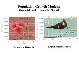
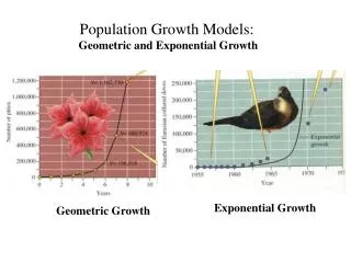
Population Growth • Geometric growth • II. Exponential growth • III. Logistic growth
www.smalltownproject.org/ Bottom line: • When there are no limits, populations grow faster, • and FASTER • and FASTER!
Invasive Cordgrass (Spartina) in Willapa Bay http://two.ucdavis.edu/willapa1.jpg
The Simple Case: Geometric Growth • Constant reproduction rate • Non-overlapping generations (like annual plants, insects) • Also, discrete breeding seasons (like birds, trees, bears) • Suppose the initial population size is 1 individual. • The indiv. reproduces once & dies, leaving 2 offspring. • How many if this continues?
Equations for Geometric Growth • Growth from one season to the next: Nt+1 = Nt, where: • Nt is the number of individuals at time t • Nt+1 is the number of individuals at time t+1 • is the rate of geometric growth • If > 1, the population will increase • If < 1, the population will decrease • If = 1, the population will stay unchanged
Equations for Geometric Growth • From our previous example, = 2 • If Nt = 4, how many the next breeding cycle? • Nt+1 = Nt = (4)(2) = 8 • How many the following breeding cycle? • Nt+1 = (4)(2)(2) = 16 • In general, with knowledge of the initial N and , • one can estimate N at any time in the future by: • Nt = N0 t
Using the Equations for Geometric Growth • If N0 = 2, = 2, how many after 5 breeding cycles? • Nt = N0 t = (2)(2)5 = (2)(32) = 64 • If N0 = 1000, = 2, how many after 5 breeding cycles? • Nt = N0 t = (1000)(2)5 = (1000)(32) = 32,000
What does “faster” mean? • Growth rate vs. number of new individuals
Using the Equations for Geometric Growth • If in 2001, there were 500 black bears in the Pasayten Wilderness, and there were 600 in 2002, how many would there be in 2010? • First, estimate : • If Nt+1 = Nt , then = Nt+1/Nt, or 600/500 = 1.2 • If N0 = 500, = 1.2, then in 2010 (9 breeding cycles later) • N9 = N0 9 = (500)(1.2)9 = 2579 • In 2060 (59 breeding seasons), N = 23,478,130 bears!
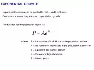
Exponential Growth - Continuous Breeding dN/dt = rN, where dN/dt is the instantaneous rate of change r is the intrinsic rate of increase
Exponential Growth - Continuous Breeding r explained: r = b - d, where b is the birth rate, and d is the death rate Both are expressed in units of indivs/indiv/unit time When b>d, r>0, and dN/dt (=rN) is positive When b<d, r<0, and dN/dt is negative When b=d, r=0, and dN/dt = 0
Equations for Exponential Growth • If N = 100, and r = 0.1 indivs/indiv/day, how much growth in one day? • dN/dt = rN = (0.1)(100) = 10 individuals • To predict N at any time in the future, one needs to solve the differential equation: • Nt = N0ert
Exponential Growth in Rats • In Norway rats that invade a new warehouse with ideal conditions, r = 0.0147 indivs/indiv/day • If N0 = 10 rats, how many at the end of 100 days? • Nt = N0ert, so N100 = 10e(0.0147)(100) = 43.5 rats
Comparing Exponential and Geometric Equations: • Geometric: Nt = N0t • Exponential: Nt = N0ert • Thus, a reasonable way to compare growth parameters is: er = , or r = ln()
Assumptions of the Equations • All individuals reproduce equally well. • All individuals survive equally well. • Conditions do not change through time.
A. Body size and r • On average, small organisms have higher rates of per capita increase and more variable populations than large organisms. 11.21
Small and fast vs. large and slow TUNICATES: Fast response to resources • WHALES: • Reilly et.al.used annual migration counts from 1967-1980 to obtain 2.5% annual growth rate. • Thus from 1967-1980, pattern of growth in California Gray Whale pop fit exponential model: • Nt = No e0.025t 11.22
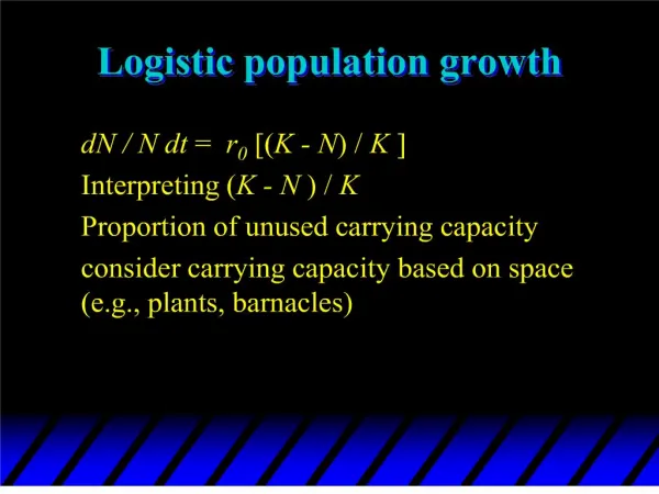
What happens if there ARE limits? (And eventually there ALWAYS are!) • LOGISTIC POPULATION GROWTH