Download
1 / 45
450 likes | 568 Views
Dow Jones and Oil Prices. ECON 240C Take Home 2 Members: Jessica Aguirre Edward Han Masatoshi Hirokawa Han Liu Lu Mao Christian Mundo Yuejing Wu. Contents. Part A: Introduction Part B: The 1973-1974 oil crisis Part C: Pre-whitening oil price (oilp)

E N D
Dow Jones and Oil Prices ECON 240C Take Home 2 Members: Jessica Aguirre Edward Han Masatoshi Hirokawa Han Liu Lu Mao Christian Mundo Yuejing Wu
Contents • Part A: Introduction • Part B: The 1973-1974 oil crisis • Part C: Pre-whitening oil price (oilp) • Part D: Transforming first differenced Dow Jones Average (ddji) to W • Part E: Fitting a distributed lag model • Part F: Forecasting the Dow Jones Industrial Average
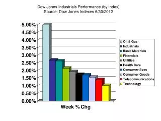
Introduction • The impact of oil prices on the stock marketis inversely proportional. An increase in oil prices leads to a decrease in the stock market. On the contrary, a decrease in oil price on average leads to a higher stock market return. • We assume that the effect of oil prices can be predictable in the stock market. • We used following monthly data from January 1946 to April 2011. • The Spot Oil Price: West Texas Intermediate (adjusted to real oil price) • The Dow Jones Industrial Average.
1973-74 Oil Crisis Part 1 • In October of 1973 Middle-eastern OPEC nations stopped oil exports to the US and other western nations. They meant to punish the western nations that supported Israel. • Prices of gasoline quadrupled, rising from just 25 cents to over a dollar per gallon in just a few months. • The American Automobile Association recorded that up to twenty percent of the country’s gas stations had no fuel one week during the crisis and drivers were forced to wait in line for 2-3 hours to get gas.
1973-74 Oil Crisis Part 2 • The total consumption of oil in the U.S. dropped twenty percent due to the effort of the public to conserve oil and money. • The embargo ended in 1974 and Arabs began to ship oil to Western nations again, but at inflated prices. • Therefore, there is a huge gap with oil price in 1973.
Oil Prices • Oil prices for 1946 to 2010 (taken monthly) • Notice the change in habit around 1973-1974 • Before 1973 Oil prices remained extremely stable
Normality (OILP) • Using a histogram we can show that OILP is not Normal • Jaque-Bera: 177.94 • Probability: 0.0000 • This breaks an assumption of the OLS Model
Correlation (OILP) • Autocorrelation shows signs of an evolutionary model • This may be the result of a unit root
ADF Test (OILP) • The ADF test shows that the unit root null hypothesis can not be rejected
First Difference of Oil Prices • In an attempt to remove the unit root we take the first difference of OILP • The resulting graph looks much less evolutionary
Normality (DOILP) • Jarque Bera: 108202 • Probability: 0.0000 • Kurtosis: 60.08 • Skewness: 3.8088
Correlation (DOILP) • Partial Correlation significant lags are: • 4 • 6 • 12 • 15 • 16 • This translates into: • AR(4) • AR(6)
Unit Test (DOILP) • ADF Test Statistic • -26.369 • 1% Level: -3.44 • 5% Level: -2.87 • 10% Level:-2.57 • No Unit root
Estimation (DOILP) • Estimated Equation: DOILP = AR(4) + AR(6) + C • DOILP(t)=-0.0968*DOILP(t-4)-0.0626*DOILP(t-6)+N(t) • N(t) = (1+0.0968*Z4+ 0.0626*Z6)*DOILP(t)
Testing Residuals • The correlelogram shows a satisfactory form • Slight structure at lag 15, but nothing to be concerned of
Testing for ARCH Residuals • When testing for the Residuals squared we can see that there is no significant lags
Distributed Lag Model for DJI(t) • dji(t) = h(z) oilp(t) + residdji(t) • Take first difference • ddji(t) = h(z) doilp(t) + dresiddji(t) • Multiply by our estimated model • (1+0.0968*Z4+0.0626*Z6)*doilp(t)=Ndoilp(t) • W(t) = h(z) Ndoilp (t) + residw(t) • Where • W(t) = (1+0.0968*Z4+0.0626*Z6) ddji(t) • residw(t) = (1+0.0968*Z4+0.0626*Z6) dresiddji(t)
Part C: Transforming DDJI to W(t) • DJI, unlike oil prices does not spikes and change in volatility in 1973 – 1974
Normality (DJI) • Jarque Bera: 208 • Probability: 0.000 • Kurtosis: 3.00 • Skewness: 1.264 • Non-normal distribution
Correlation DJI • Autocorrelation shows signs of evolutionary data
ADF Test (DJI) • T-statistic: 0.57 • 1% Level: -3.43 • 5% Level: -2.87 • 10% Level: -2.5 • Shows signs that there exists a unit root
First Difference DDJI • To remove the evolutionary aspects of DJI we take the first difference
Normality (DDJI) • Jarque Bera: 15024 • Probability: 0.000 • Kurtosis: 24.10 • Skewness: -1.96
ADF Test (DDJI) • T-statistic -10.42 • 1% Level -3.44 • 5% Level -2.87 • 10% Level -2.57 • Reject unit root
Fit DDJI to W • W(t) = (1 + 0.0968*Z^4 + 0.0626*Z^6) DDJI(t)
Normality (W(t)) • Jarque Bera: 15233.9 • Skewness: -1.953 • Kurtosis: 24.34
ADF Test (W) • T-statistic: -10.02 • 1% Level -3.44 • 5% Level -2.87 • 10% Level -2.57
Part E : fitting a distributed lag model DOILP CAUSES DDJI
Part E : fitting a distributed lag model Lags 3,11, 13, 29 are significant
Part F: Forecasting • Forecasting: 2011m05 2011m06
Forecasting (continued) • 150.1134+/- 2*180.2 (-210.3~510.5) • 143.4469+/- 2*180.2 (-216.9~503.8) • The value for April 2011 is 12434.88 • dji(2011.5)=12434.88+150.1134=12584.9934, about 12585 (12224.58~12945.38) • Real value for 2011.05 • 12587.81 only 2.81 points difference! • Forecasting for June 2011: • Dji(2011.6)= 12587.81+143.4469=12731.2569 (12370.86~13091.61)