Download
1 / 55
550 likes | 699 Views
Soft Error Benchmarking of L2 Caches with PARMA. Jinho Suh Mehrtash Manoochehri Murali Annavaram Michel Dubois. Outline. Introduction Soft Errors Evaluating Soft Errors PARMA: Precise Analytical Reliability Model for Architecture Model Applications Conclusion and Future work.

E N D
Soft Error Benchmarking of L2 Caches with PARMA Jinho Suh Mehrtash Manoochehri MuraliAnnavaram Michel Dubois
Outline • Introduction • Soft Errors • Evaluating Soft Errors • PARMA: Precise Analytical Reliability Model for Architecture • Model • Applications • Conclusion and Future work
Outline • Introduction • Soft Errors • Evaluating Soft Errors • PARMA: Precise Analytical Reliability Model for Architecture • Model • Applications • Conclusion and Future work
Soft Errors • Random errors on perfect circuits, mostly affect SRAMs • From alpha particles (electric noises) • From neutron strikes in cosmic rays • Severe problem, especially with power saving techniques • Superlinear increases with Voltage & Capacitance scaling • Near-/sub-threshold Vdd operation for power savings • Concerns in: • Large servers • Avionic or space electronics • SRAM caches with drowsy modes • eDRAM caches with reduced refresh rates
Why Benchmark Soft Errors • Designers need good estimation of expected errors to incorporate ‘just-right’ solution at design time • Good estimation is non-trivial • Multi-Bit Errors are expected • Masking effects: Not every Single Event Upset leads to an error [Mukherjee’03] • Faults become errors when they propagate to the outer scope • Faults can be masked off at various levels • Design decision • When the protection under consideration is too much or too little? • Is a newly proposed protection scheme better? • The impact of soft errors needs to be addressed at design time • Estimating soft error rates for target application domains is an important issue
Evaluating Soft Errors:Some Reliability Benchmarking Approaches • Fundamental difficulty: Soft errors happen very rarely Field Analysis Life Testing • Intrinsic FIT (Failure-in-Time) rate • Highly pessimistic: no consideration of masking effects • Unclear for protected caches • AVF [Mukherjee’03] and SoftArch[Li’05] • Quickly compute SDC without protection or DUE under parity • Ignores temporal/spatial MBEs • Can’t account for error detection/correction schemes • Difficulty in collecting data • Obsolete for design iteration [Ziegler] Fault Injection Accelerated Testing • Require massive experiments • Distortion in measurement/interpretation Analytical Modeling Intrinsic SER AVF SoftArch • Better for estimating SER in short time • Complexity determines preciseness
Outline • Introduction • Soft Errors • Evaluating Soft Errors • PARMA: Precise Analytical Reliability Model for Architecture • Model • Applications • Conclusion and Future work
Two Components of PARMA (Precise Analytical Reliability Model for Architecture) • Fault generation model • Fault propagation model • Fault becomes Error when faulty bit is consumed • Instruction with faulty bit commits • Load commits and its operand has a faulty bit Poisson Single Event Upset model Probability distribution of having k faulty bit(s) in a domain (set of bits) during multiple cycles • PARMA measures: • Generated faults Propagated faults Expected errors Error rate
Using Vulnerability Clocks Cycles to Track Bit Lifetime • Used to track cycles that any bit spends in vulnerable component: L2$ • Ticks when a bit resides in L2 • Stops when a bit stays outside L2 • Similar to lifetime analysis in AVF method Word# Word# Word# Word# VC VC VC VC When a word is updated to hold new data, its VC resets to zero When this block is refilled later, VCs should start ticking from here 0 0 0 0 100 500 200 0 1 1 1 1 0 300 0 100 2 2 2 2 500 100 200 0 3 3 3 3 0 200 500 100 Proc Main Memory L1$ L2$ VC: ticks VC: stops Set of bits Set of bits Accesses to L1$ determines REAL impact of Soft Error to the system L2 block is NOT dead even when it is evicted to MEM because it can be refilled into L2 later When L1 block is evicted, consumption of the faulty bits is finalized
Probability of a Bit Flip in One Cycle • SEU Model • p : probability that one bit is flipped during one cycle period • Poisson probability mass function gives p • λ: Poisson rate of SEUs • ex) 10-25/bit @ 65nm 3GHz CPU
Temporal Expansion: Probability of a Bit Flip in Nc vulnerability cycles • q(Nc) : probability of a bit being faulty in Ncvulnerability cycles • To be faulty at the end of Nc cycles, a bit must flip an odd number of times in Nc
Spatial Expansion: from a Bit to the Protection Domain (Word) • SQ(k) • Probability of set of bits Shaving k faulty bits inside (during Nc cycles) • Choose cases where there are k faulty bits in S • S has [S] bits inside • Assumed that all the bits in the word have the same VCs • Otherwise, discrete convolution should be used
Faults in the Access Domain (Block) • DQ(k) • Probability of k faulty bits in any protection domain inside of D (Sm) • Choose cases where there are k faulty bits in each Sm • Sum for all Sm in D • So far, masking effect has not been considered • Expected number of intrinsic faults/errors are calculated so far
Considering Masking Effect: Separating TRUE from Intrinsic Faults • If all faults occur in unconsumed bits, then don’t care (FALSE events) • TRUE faults = {All faults in S} – {All faults in unconsumed bits} • Probability that has k faults, and C has 0 fault: FALSE or masked faults • Deduct the probability that ALL k faulty bits are in the unconsumed bytes from the probability that the protection domain S has k faulty bits to obtain the probability of TRUE faults which becomes SDCs or TRUE DUEs • C and are obtained through simulations
Using PARMA to Measure Errors in Block Protected by block-level SECDED 2 faults in Block >=3 faults in Block • Undetected error that affects reliability (SDC): three or more faulty bits in the block; at least one faulty bit in the consumed bits • Detected error that affects reliability (TRUE DUE): exactly two faulty bits in the block; at least one faulty bit in the consumed bits k>=3 is SDC k =2 is DUE All faulty bits unconsumed All faulty bits unconsumed See paper for how to apply PARMA on the different protection schemes
Four Contributions • Development of the rigorous analytical model called PARMA • Measuring SERs on structures protected by various schemes • Observing possible distortions in the accelerated studies • Quantitatively • Qualitatively • Verifying approximate models Modeling Application
Measuring SERs on Structures Protected by Various Schemes • Target Failures-In-Time of IBM Power6 • SDC: 114 • DUE: 4,566 • Average L2 (256KB, 32B block) cache FITs: • 100M SimPoint simulations of 18 benchmarks from SPEC2K, on sim-outorder • Implies word-level SECDED might be overkill in most cases • Implies increasing the protection domain size: ex) CPPC @ISCA2011 • Partially protected caches or caches with adaptive protection schemes need to be carefully quantified for their FITs • PARMA provides comprehensive framework that can measure the effectiveness of such schemes Results were verified with AVF simulations
Observing Possible Distortions in the Accelerated Tests • Highly accelerated tests • SPEC2K benchmarks end in several minutes (wall-clock time) • Needs to accelerate SEU rate 1017 times to see reasonable faults MAX Possible Errors • How to scale down the results? • Results multiplied by 10-17 times? • Can distort results quantitatively DUE • SDC > DUE ? • Having more than two errors overwhelms the cases of having two errors • Can be misleading qualitatively SDC Results were verified with fault-injection simulations
Verifying Approximate Models • Example: model for word level SECDED protected cache • Methods for determining cache scrubbing rates[Mukherjee’04][Saleh’90] • Ignoring cleaning effects at accesses: overestimate by how much? • New model with geometric distribution of Bernoulli trials • Assumption: at most two bits are flipped between two accesses to the same word • Every access results in a detected error or in no-error (corrected) New approximate model 2.8246E-14 FIT PDUE: pmf of two Poisson arrivals AVF x FIT from previous method 2.1454 FIT Average ACE interval Average unACE interval PARMA 6.3170E-16 FIT TAVG: Average access interval between two accesses to the same word Mean of geometric distribution • PARMA provides rigorous reliability measurements • Hence, it is useful to verify the faster, simpler approximate models
Outline • Introduction • Soft Errors • Evaluating Soft Errors • PARMA: Precise Analytical Reliability Model for Architecture • Model • Applications • Conclusion and Future work
Conclusion and Future Work • Summary • PARMA is a rigorous model measuring Soft Error Rates in architectures • PARMA works with wide range of SEU rates without distortion • PARMA handles temporal MBEs • PARMA quantifies SDCor DUE rates under various error detection/protection schemes • PARMA does not address spatial MBEs yet • PARMA does not model TAG yet • Due to the complexity, PARMA is slow • Future Work • Extend PARMA to account for spatial MBEs and TAG vulnerability • Develop sampling methods to accelerate PARMA
(Some) References [Biswas’05] A. Biswas, P. Racunas, R. Cheveresan, J. Emer, S. Mukherjee, R Rangan, Computing Architectural Vulnerability Factors for Address-Based Structures, In Proceedings of the 32nd International Symposium on Computer Architecture, 532-543, 2005 [Li’05] X. Li, S. Adve, P. Bose, and J.A. Rivers. SoftArch: An Architecture Level Tool for Modeling and Analyzing Soft Errors. In Proceedings of the International Conference on Dependable Systems and Networks, 496-505, 2005. [Mukherjee’03] S. S. Mukherjee, C. Weaver, J. Emer, S. K. Reinhardt, and T. Austin. A systematic methodology to calculate the architectural vulnerability factors for a high-performance microprocessor. In Proceedings of the 36th International Symposium on Microarchitecture, pages 29-40, 2003. [Mukherjee’04] S. S. Mukherjee, J. Emer, T. Fossum, and S. K. Reinhardt. Cache Scrubbing in Microprocessors: Myth or Necessity? In Proceedings of the 10th IEEE Pacific Rim Symposium on Dependable Computing, 37-42, 2004. [Saleh’90] A. M. Saleh, J. J. Serrano, and J. H. Patel. Reliability of Scrubbing Recovery Techniques for Memory Systems. In IEEE Transactions on Reliability, 39(1), 114-122, 1990. [Ziegler] J. F. Ziegler and H. Puchner, “SER – History, Trends and Challenges,” Cypress Semiconductor Corp
Some Definitions • SDC = Silent Data Corruption • DUE = Detected and unrecoverable error • SER = Soft Error Rate = SDC + DUE • Errors are measured as • MTTF = Mean Time to Failure • FIT = Failure in Time ; 1 FIT = 1 failure in billion hours • 1 year MTTF = 1billion/(24*365)= 114,155 FIT • FIT is commonly used since FIT is additive • Vulnerability Factor = fraction of faults that become errors • Also called derating factor or soft error sensitivity
Soft Errors and Technology Scaling • Hazucha & Svensson model • For a specific size of SRAM array: • Flux depends on altitude & geomagnetic shielding (environmental factor) • (Bit)Area is process technology dependent (technology factor) • Qcoll is charge collection efficiency, technology dependent • Qcrit Cnode * Vdd • According to scaling rules both C and V decrease and hence Q decreases rapidly • Static power saving techniques (on caches) with drowsy mode or using near-/sub-threshold Vdd make cells more vulnerable to soft errors Hazucha et al, “Impact of CMOS technology scaling on the atmospheric neutron soft error rate ”
Error Classification • Silent Data Corruption (SDC) • TRUE- and FALSE- Detected Unrecoverable Error (DUE) Consumed ? Consumed? C. Weaver et al, “Techniques to Reduce the Soft Error Rate of a High-Performance Microprocessor,” ISCA 2004
Soft Error Rate (SER) • Intrinsic SER – more from the component’s view • Assumes all bits are important all the time • Intrinsic SER projections from ITRS2007 (High Performance model) • Intrinsic SER of caches protected by SECDED code? • Cleaning effect on every access • Realistic SER – more from the system’s view • Some soft errors are masked and do not cause system failure • EX) AVF x Intrinsic SER: what about caches with protection code?
Soft Error Estimation Methodologies: Industries • Field analysis • Statistically analyzes reported soft errors in market products • Using repair record, sales of replacement parts • Provides obsolete data • Life testing • Tester constantly cycles through 1,000 chips looking for errors • Takes around six months • Expensive, not fast enough for chip design process • Usually used to confirm the accuracy of accelerated testing (x2 rule) • Accelerated testing • Chips under various beams of particles, under well-defined test protocol • Terrestrial neutrons – particle accelerators (protons) • Thermal neutrons – nuclear reactors • Radioactive contamination – radioactive materials • Hardship • Data rarely published: potential liability problems of products • Even rarer the comparison of accelerated testing vs life testing • IBM, Cypress published small amount of data showing correlation J. F. Ziegler and H. Puchner, “SER – History, Trends and Challenges,” Cypress Semiconductor Corp
Soft Error Estimation Methodologies: Common Ways in Researches • Fault-injection • Generate artificial faults based on the fault model • Applicable to wide level of designs (from RTL to system simulations) • Massive number of simulations necessary to be statistically valid • Highly accelerated Single Event Upset (SEU) rate is required for Soft Errors • How to scale down the measurements to ‘real environment’ is unclear • Architectural Vulnerability Factor • Find derating factor (Faults Errors) by {ACE bits}/{total bits} per cycle • SoftArch • Extrapolate AVG(TTFs) from one program to MTTF using infinite executions • AVF and SoftArch – uses simplified Poisson fault generation model • Works well with small scale system in the current technology at earth’s surface: single bit error dominant environment • Can’t account for error protection/detection schemes (ECC) • Unable to address temporal & spatial MBEs • AVF is NOT an absolute metric for reliability • FITstructure = intrinsic_FITstructure * AVFstructure M. Li et al, “Accurate Microarchitecture-Level Fault Modeling for Studying Hardware Faults,” HPCA 2009 S. S Mukherjee et al, “A systematic methodology to calculate the architectural vulnerability factors for a high-performance microprocessor.” MICRO 2003 X. Li et al, “SoftArch: An Architecture Level Tool for Modeling and Analyzing Soft Errors.” DSN 2005
Evaluating Soft Errors:Some Reliability Benchmarking Approaches • Intrinsic FIT (Failure-in-Time) rate – highly pessimistic • Every bit is vulnerable in every cycle • Unclear how to compute intrinsic FIT rates for protected caches • Architectural Vulnerability Factor [Mukherjee’03] • Lifetime analysis on Architecturally Correct Execution bits • De-rating factor (Faults Errors); realistic FIT = AVF x Intrinsic FIT • SoftArch[Li’05] • Computes TTF for one program run and extrapolates to MTTF • AVF and SoftArch • Quickly compute SDC with no parity or DUE under parity • Ignores temporal MBEs • Two SEUs on one word become two faults instead of one fault • Two SEUs on the same bit become two faults instead of zero fault • Ignores spatial MBEs • Can’t account for error detection / correction schemes • To compare SERs of various error correcting schemes: • Temporal/spatial MBEs must be accurately counted
Prior State of the Art Reliability Model: AVF • Architectural Vulnerability Factor (AVF) • AVFbit = Probability a bit matters (for a user-visible error) = # of bits affects to user-visible outcome / total # of bits • If we assume AVF = 100% then we will over design the system • Need to estimate AVF to optimize the system design for reliability • AVF equation for a target structure • AVF is NOT an absolute metric for reliability • FITstructure = intrinsic_FITstructure * AVFstructure ……(Eq. 1) Shubu Mukherjee, “Architecture design for soft errors”
ACEness of a bit • ACE (Architecturally Correct Execution) bit • ACE bit affects program outcome: correctness is subjective (user-visible) • Microarchitectural ACE bits • Invisible to programmer, but affects program outcome • Easier to consider Un-ACE bits • Idle/Invalid/Misspeculated state • Predictor structures • Ex-ACE state (architecturally dead or invisible states) • Architectural ACE bits • Visible to programmer • Transitive (ACE bit in the word makes the Load instruction ACE) • Easier to consider Un-ACE bits • NOP instructions • Performance-enhancing operations (non-opcode field of non-binding prefetch, branch prediction hint) • Predicated false instructions (except predicate status bit) • Dynamically dead instructions • Logical masking • AVF framework = lifetime analysis to correctly find ACEness of bits in the target structure for every operating cycle Shubu Mukherjee, “Architecture design for soft errors”
Rigorous Failure/Error Rate Modeling • In existing methodologies such as AVF multiplied by intrinsic rate • Estimation is simple and easy • Imprecise estimation but safe-overestimation • Downside of classical approach (i.e. AVF-based methodology) • SEU is very rare event while program execution time is rather short • In 3GHz processor, SEU rate is 1.0155E-25 within one cycle for one bit • Equivalently, the probability of being hit by SEU and being faulty bit is 1.0155E-25 • Simplified assumption that one SEU results one Fault/Error directly • same bit may be hit multiple times, and/or • multiple bits may become faulty in a word • In space, or when extremely low Vdd is supplied to SRAM cell: • SEU rate could rise high (more than 10E6 times) • Second order effects become significant • With data protection methodology: • How to measure vulnerability is uncertain due to the simplified assumption
Reliability Theory (1) • Fundamental definition of probability in Reliability Theory • Number(Event)/Number(Trials): Approximations of true Prob(Event) • True probability is barely known • approx true when trials ∞ by the Law of Large Numbers • Two events in R-T: Survival & Failure of a component/system • Reliability Functions • (Component/system) Reliability R(t), and Probability of Failure Q(t) • Prob(Event) up to and at time t: conditional probability • Note that R(t), Q(t) are time dependent in general • (Conditional) Instantaneous Failure Rate λ(t) - a.k.a, Hazard function h(t)
Reliability Theory (2) • Reliability functions (cont’d) • (Unconditional) Failure Density Function f(t) • Average Failure Rate from time 0 to T • Discrete dual of λ(t) - Hazard Probability Mass Function h(j) • Average Failure Rate from timeslot 0 to T
Reliability Theory (3) • How to measure Reliability • R(t) itself • Events with constant failure rate • MTTF • Sampling issue: Usually no test can aggregate total test time to ∞ • (Right) censorship with no replacement, then Maximum Likelihood Estimation • by B. Epstein, 1954 • At the end of the test time tr, measure TTFs (ti) for samples that failed and truncate the lifetime of all survived samples to tr • Then, MLE of MTTF is • FIT – one intuitive form of failure rate • Failures in time 1E9 hours • Interchangeable with MTTF only when failure rate is constant • Additive between independent components
Vulnerability Clock • Used to track cycles that any bit spends in vulnerable component: L2$ • Ticks when a bit resides in L2 • Stops when a bit stays outside L2 Cold Miss Store Writeback VC_MEM = 0 VC_MEM = 80 VC_MEM := VC_L2 = 80 VC_L2 = 0 VC_L2 = 0 VC_L2 = 100 VC_L2 := VC_L1= 0 VC_L2 = 1 VC_L2 = 150 VC_L2 = 80 VC_L2 := VC_MEM = 80 VC_L1 := VC_L2 = 0 VC_L1 := 0 VC_L1 = 0
PARMA Model:Measuring Soft Error FIT with PARMA • PARMA measures failure rate by accumulating failure probability mass • Index processor cycle by j (1 ≤ j ≤Texe) • Total failures observed during Texe(failure rate): • Equivalent to expected number of failures of type ERR • FIT extrapolation with infinite program execution assumption • How to calculate ? • Let’s start with p: probability that one bit is flipped during one cycle period • Obtained from Poisson SEU model
PARMA Model:Fault Generation Model • SEU Model • Assumptions: • All clock cycles are independent to SEUs • All bits are independent to SEUs (do not account for spatial MBEs) • Widely accepted model for SEU: Poisson model • p : probability that one bit is flipped during one cycle period (in SBE cases) • Spatial MBE case: probability that multi-bits become faulty during one cycle • Poisson probability mass function gives p • λ: Poisson rate of SEUs, ex) 10-25/bit @ 65nm 3GHz CPU
PARMA Model:Measuring Soft Error FIT with PARMA • PARMA measures failure rate by accumulating failure probability mass • Index processor cycle by j (1 ≤ j ≤Texe) • A (conditional) failure probability mass at cycle j : • Total failures observed during Texe(failure rate): • Equivalent to expected number of failures of type ERR • FIT extrapolation with infinite program execution assumption • Average FIT with multiple programs
Failures Measured in PARMA • No-protection, 1-bit Parity, 1-bit ECC on Word and 1-bit ECC on Block
Spatial Expansion: From a Bit to a Byte in NcVulnerability Cycles • qb(k) • Probability of a Byte having k faulty bits (in Ncvulnerability cycles) • From 8 bits in the Byte, choose k faulty bit
Spatial Expansion: from a Byte to the Protection Domain (Word) • SQ(k) • Probability of set of bits Shaving k faulty bits inside (during Nc cycles) • Choose cases where there are k faulty bits in S • Enumerate all possibilities of faulty bits in bytes of S such that their total number = k
Faults in the Access Domain (Block) • DQ(k) • Probability of k faulty bits in any protection domain inside of D (Sm) • Choose cases where there are k faulty bits in Sm • Sum for all Sm in D • So far, masking effect has not been considered • Expected number of intrinsic faults/errors are calculated so far
PARMA Model:Failures Measured in PARMA (1) • Odd parity per block • SDCs: having at least one faulty bit in the consumed bytes, from having nonzero, even number of faulty bits in the block • TRUE DUEs: having at least one faulty bit in the consumed bytes, from having odd number of faulty bits in the block • Unprotected cache • Without protection, any non-zero faulty bit(s) will cause SDC failure • SDCs: having at least one faulty bit in the consumed bits Nonzero, even # k faulty bits in the block is SDC All faults Unconsumed
PARMA Model:Failures Measured in PARMA (2) • SECDED per block • SDCs: having at least one faulty bit in the consumed bits, from having more than two faulty bits in the block • TRUE DUEs: having at least one faulty bit in the consumed bits, from having exactly two faulty bits in the block • SECDED per word • Same to ‘per block’ case except protection domain is word • Because access domain is block, all the words in the same block are addressed by adding FITs >=3 faults in Block For all the words in the block Additive because FITs from each word is independent and counted separately All faults Unconsumed k>=3 is SDC
PARMA Simulations • Target processor • 4-wide OoO processor • 64-entry ROB • 32-entry LSQ • McFarling’s hybrid branch predictor • Cache configuration • sim-outorder was modified and executed with alpha ISA • 18 benchmarks from SPEC2000 were used with SimPoint Sampling of 100M-instruction samples
Evaluating Soft Errors: AVF or Fault-Injection, Why Not? • AVF fails for handling scenarios under error protection schemes • Why not use fault injection for such scenarios? • Possible distortion in the interpretation of results due to the highly accelerated experiments