Download
1 / 23
260 likes | 676 Views
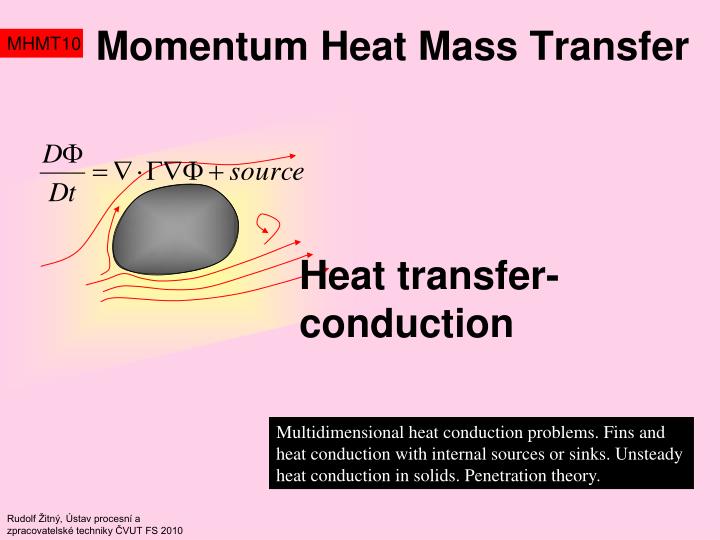
Momentum Heat Mass Transfer. MHMT 10. Heat transfer-conduction. Multidimensional heat conduction problems. Fins and h eat conduction with internal sources or sinks. Unsteady heat conduction in solids. Penetration theory. Rudolf Žitný, Ústav procesní a zpracovatelské techniky ČVUT FS 2010.

E N D
Momentum Heat Mass Transfer MHMT10 Heat transfer-conduction Multidimensional heat conduction problems. Fins and heat conduction with internal sources or sinks. Unsteady heat conduction in solids. Penetration theory. Rudolf Žitný, Ústav procesní a zpracovatelské techniky ČVUT FS 2010
Heat transfer - conduction 1 Tf1 Tf2 2 2 1 D1 Dm D2 MHMT10 Thermal resistance of fluid (thermal boundary layer) can be expressed in terms of heat transfer coefficients added to the thermal resistances of solid layers. For example resulting RT of serial resistances of fluid and two concentric pipes can be expressed as (see previous lecture) Example (critical thickness of insulation): Let us assume that only the thickness of insulation (outer diameter D2) can be changed. Then the thermal resistance (and effectiveness of insulation) depends only upon D2, see graph calculated for D1=0.02 m, Dm=0.021, 1=40 W/(m.K) (steel), 2=0.1 (insulation), 1=1000, 2=5 (natural convection) . Up to a critical D2 the thermal resistance DECREASES with the increasing thickness of insulation!
Heat transfer - conduction 1 Tf1 2 Tf2 1 2 D1 Dm D2 MHMT10 Thermal resistance of a composite tube with circular or spiral fins attached to outer tube (fins can be also an integral part of the outer tube). Resulting thermal resistance is calculated according to almost the same expression as in the previous case with the only but very important difference: Instead of the outer surface of plain tube D2L is used the overall outer surface of fins S2L. Such a modification assumes that the 2 on the surface of fins is the same as on the surface of tube and first of all that the thermal resistance of fin itself is negligible (simple speaking it is assumed that the fin is made of material having infinite value of thermal conductivity ).
Heat transfer - conduction Tw , Tf b T(x) dx x H MHMT10 The assumption of perfectly conductive fin is unacceptable and in reality the thermal resistance of fin must be respected by multiplying the surface S2 by fin’s efficiency fin which depends upon thermal conductivity of fin, its geometry (thickness and height) and also upon the heat transfer coefficient 2. Efficiency of a thin rectangular fin can be derived easily by solution of temperature profile along the height of fin This is FK equation with a source term, representing heat transfer from both sides of surface (2dx) to the control volume (bdx) with boundary conditions at the heel of fin (T(x=0)=Tw) and at top of fin dT/dx=0 (there is no heat flux at x=H) Efficiency of fin is calculated from temperature gradient at the heel of fin (the gradient determines heat flux at the heel)
Conduction - nonstationary MHMT10
Conduction - nonstationary MHMT10 Temperature distribution in unsteady case generally depends upon time t and coordinates x,y,z. Sometimes, when the temperature distribution is almost homogeneous inside the whole body, the partial differential Fourier Kirchhoff equation reduces to an ordinary differential equation. This simplification is correct if the thermal resistance of solid is much less than the thermal resistance of fluid, more specifically if Biot number is small enough here D is a characteristic diameter of a solid object and s is thermal conductivity of solid Fourier Kirchhoff equation can be integrated over the whole volume of solid which reduces to ordinary dif. equation as soon as Ts depends only on time
Conduction - nonstationary MHMT10 As soon as the Biot number is large (Bi>0.1, therefore if the solid body is too big, for example semi-infinite space) it is necessary to solve the parabolic partial differential Fourier Kirchhoff equation. For the case that the solid body is homogeneous (constant thermal conductivity, density and specific heat capacity) and without internal heat sources the FK equation reduces to with the boundary conditions of the same kind as in the steady state case and with initial conditions (temperature distribution at time t=0). This solution T(t,x,y,z) can be expressed for simple geometries in an analytical form (heating brick, plate, cylinder, sphere) or numerically in case of more complicated geometries. The coefficient of temperature diffusivity a=/cpis the ratio of temperature conductivity and thermal inertia
Conduction - nonstationary Tw t x T0 δ MHMT10 Start up flow of viscous liquid in halfspace (solved in lecture 4) was described by equation which is identical with the Fourier Kirchhoff equation for one dimensional temperature distribution in halfspace and with the step change of surface temperature as a boundary condition: T(t=0,x)=T0 T(t,x=0)=Tw Exactly the same solution as for the start up flow (complementary error function erfc) holds for dimensionless temperature
Conduction - nonstationary Tw() x d MHMT10 Erfc function describes temperature response to a unit step at surface (jump from zero to a constant value 1). The case with prescribed time course of temperature at surface Tw(t) can be solved by using the superposition principle and the response can be expressed as a convolution integral. t Temperature at a distance x is the sum of responses to short pulses Tw()d Time course Tw(t) can be substituted by short pulses The function E(t,,x)=E(t-,x) is the impulse function (response at a distance x to a temperature pulse of infinitely short duration but unit area – Dirac delta function). The impulse response can be derived from derivative of the erfc function
Penetration theory Tw t+t t x T0 δ +Δ MHMT10 Still too complicated? Your pocket calculator is not equipped with the erf-function? Use the acceptable approximation by linear temperature profile, (exactly the same procedure as with the start up flow in a half-space) Integrate Fourier equations (up to this step it is accurate) Approximate temperature profile by line Result is ODE for thickness as a function of time Using the exact temperature profile predicted by erf-function, the penetration depth slightly differs =(at)
Penetration theory MHMT10 =at penetration depth. Extremely simple and important result, it gives us prediction of how far the temperature change penetrates at the time t. This estimate enables prediction of thermal and momentum boundary layers thickness etc. The same formula can be used for calculation of penetration depth in diffusion, replacing temperature diffusivity a by the diffusion coefficient DA . Wire Cu =0.11 m =398 W/m/K =8930 kg/m3 Cp=386 J/kg/K
Penetration theory and Tf Tw t+t t x T0 δ +Δ MHMT10 The penetration theory can be applied also in the case that the semi-infinite space is in contact with fluid and surface temperature depends upon temperature of fluid and the heat transfer coefficient Derive the result as a homework
PLATE - finite depth Bi<0.1 Bi1 Bi Tf Tf Tw=Tf Fo>1 Fo>1 Tw Tw Fo<1 Fo<1 T0 T0 T0 H/2 H/2 H/2 x MHMT10 In case of a finite thickness plate the penetration theory can be used only for short times (small Fourier number < 0.1) Let us define Fourier number and Biot number in terms of half thickness of plate H/2 Long times (large Fourier) and finite Biot.. The most complicated case/see next slide Integral method Fourier method Penetration theory
PLATE - finite depth Fourier method Bi1 Tf Tw t T0 x H/2 MHMT10 Using dimensionless temperature , distance , time (Fourier number) and dimensionless heat transfer coefficient Bi (Biot number) the Fourier Kirchhoff equation, boundary and initial conditions are transformed to Fourier method is based upon superposition of solutions satisfying differential equation and boundary conditions
PLATE - finite depth MHMT10 Spatial component Gi() follows from The function cos() automatically satisfies the boundary condition at =0 for arbitrary . The boundary condition at wall is satisfied only for yet undetermined values , roots of transcendental equation and this equation must be solved numerically, giving infinite series of roots 1, 2,… These eigenvalues i determine also the temporary components Fi Final temperature distribution is the infinite series of these elementary solutions
PLATE - finite depth MHMT10 The coefficients ci are determined by the initial condition To solve the coefficients ci from this identity (which should be satisfied for arbitrary ) it is convenient to utilise orthogonality of functions Gi() and Gj() that follows from original ordinary differential equations and boundary conditions for ij therefore giving final temperature profile
PLATE/CYLINDER/SPHERE MHMT10 Unsteady temperature profiles inside a sphere and infinitely long cylinders can be obtained in almost the same way, giving temperature profiles in form of infinite series where and only eigenvalues I have to be calculated numerically. This form of analytical solution is especially suitable for description of temperature field at longer times, because exponential terms quickly decay and only few terms in the series are necessary. For shorter times the penetration theory can be applied effectively This analytical solution is presented in the book Carslaw H.S., Yeager J.C.: Conduction of Heat in Solids. Oxford Sci.Publ. 2nd Edition, 2004
3D – brick,finite cylinder… y x hy hx MHMT10 It is fantastic that an unsteady temperature field in the finite 2D or 3D bodies can be obtained in the form of PRODUCT of 1D solutions expressed in terms of dimensionless temperatures x yz !!! For example the temperature distribution in an infinitely long rod with rectangular cross section hx x hy is calculated as Proof: …and you see that the FK equation is satisfied if x y are solutions of 1D problem.
3D – excercise MHMT10 Calculate temperature in the center of a cube Calculate temperature in the corner using erfc solution y x
EXAM MHMT10 Fins and Unsteady heat conduction
What is important (at least for exam) MHMT10 Thermal resistance of finned tube Efficiency of a planar fin
What is important (at least for exam) MHMT10 Unsteady heat conduction Transient heating of a semi-infinite space Simplified solution by penetration depth Temperature response to variable surface temperature
What is important (at least for exam) MHMT10 Find solution of equation for Dirichlet boundary condition at =1 and Neumann boundary condition at =0 Why is it necessary to use dimensionless temperatures in the “product” solution of 2D and 3D problems?