Introduction to Probability

1. Introduction to Probability Chapter 6

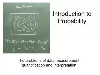
2. Introduction • In this chapter we discuss the likelihood of occurrence for events with uncertain outcomes. • We define a scale to measure and describe the chance that different outcomes of an uncertain event will take place. • This ‘measure of uncertainty’ called “Probability” serves as the basis for the analysis and results discussed at the rest of this course.

3. 6.1 Assigning probabilities to Events • Random experiment • a random experiment is a process or course of action, whose outcome is uncertain. • ExamplesExperiment Outcomes • Flip a coin Heads and Tails • The marks of a statistics test Numbers between 0 and 100 • The time to assemble Non-negative numbersa computer

4. 6.1 Assigning probabilities to Events • Because of the random nature of the experiment, repeated experiments may result in different outcomes. Consequently, one cannot refer to the experiment outcome in certain terms, only in terms of the probability of each outcome to occur. • To determine the probabilities we need to define and list the possible outcomes first. Such a list should be • exhaustive (list of all the possible outcomes). • the outcomes are mutually exclusive (outcome do not overlap). • A list of outcomes that meet the two conditions above, is called asample space.

5. O1 O2 Sample Space: S = {O1, O2,…,Ok} Sample Space a sample space of a random experiment is a list of all possible outcomes of the experiment. The outcomes must be mutually exclusive and exhaustive. Simple events The individual outcomes are called simple events. Simple events cannot be further decomposed into constituent outcomes. Event An event is any collection of one or more simple events

6. Sample Space: S = {O1, O2,…,Ok} Our objective is to determine P(A), the probability that event A will occur.

7. Sample Space: S = {O1, O2,…,Ok} Example 1: Build the sample space for the two random experiments described below • Case 1: A ball is randomly selected from an urn containing blue and red balls. An outcome is considered the ball color. The sample space: {B, R} • Case 2: Two balls are randomly selected from an urn that contains blue and red balls. An outcome is considered the colors of the two balls drawn. The sample space: {BB, BR, RB, RR}

8. Sample Space: S = {O1, O2,…,Ok} • Example 2: Build the sample space for the random experiment defined by the random selection of two numbers from the set 1, 2, 3, 4, 5 (a number cannot be selected twice). An outcome is defined by the sum of the two numbers. 1+5, 2+4 3+5 1+3 The sample space: {3, 4, 5, 6, 7, 8, 9} 2+5, 3+4 1+2 1+4, 2+3; 4+5

9. 6.1 Assigning probabilities to Events • Given a sample space S={O1,O2,…,Ok}, the following characteristics for the probability P(Oi) of the experimental outcome Oi must hold: • The probability of an event: The probability P(A) of event A is the sum of the probabilities assigned to the simple events contained in A.

10. Approaches to Assigning Probabilities and interpretation of Probability • Approaches • The classical approach • The relative frequency approach • The subjective approach

11. Events and their Probabilities • An event is a collection of sample points. • Example 3: A dice is rolled once. The following events are defined. Specify the sample points that belong to each event.Event A = the number facing up is 6 Event B = The number facing up is odd Event C = The number facing up is not greater than 4Solution: A = {6}; B = {1, 3, 5}; C = {1, 2, 3) • Example 4: A dice is rolled once and the outcome is 3.Which event takes place?Solution: Event B and event C take place because the outcome ‘3’ belongs to both events.

12. Probability of an Event Example 5:A dice is rolled once. Each number is equally likely to face up. Find the probabilities of the following events:Event A = the number facing up is 6 Event B = The number facing up is odd Event C = The number facing up is not greater than 4 Solution: P(A) = P{6} = 1/6;P(B) = P(1 or 3 or 5) = 3/6P(C) = P(1 or 2 or 3) = 3/6

13. Probability of an Event Example 6: A dice is rolled twice: Define the following events:D = The numbers facing up are the same and evenE = The sum of the two numbers facing up is 5.Define the sample space and calculate the probabilities of events D and E.SolutionThe sample space: S = {(1,1); (1,2);….(6,5); (6,6)}P(D) = P{(2,2) or (4,4) or (6,6)} = 3/36 P(E) = P{(1,4) or (2,3) or (3,2) or (4,1)} = 4/36. Note: there are 36 points in the sample space.

14. 6.2 Joint, Marginal, and Conditional Probability • Determining the probability of an event involves the counting process of its simple events. Often this may become quite cumbersome. • Understanding relationships among events may reduce the computational effort involved in determining the probability of combined events. • Combined events and there probabilities are discussed next

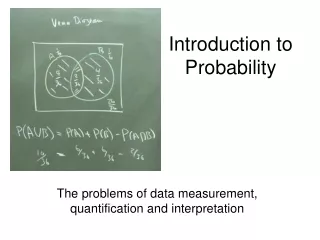
15. B A Intersection and Joint Probability • The intersection of event A and B is the event that occurs when both A and B occur. C

16. Intersection and Joint Probability • The intersection of events A and B is denoted by “A and B” ( ). • The probability of the intersection of A and B is called also the joint probability of A and B = P(A and B).

17. Intersection and Joint Probability • Example 9 • A potential investor examined the relationship between the performance of mutual funds and the school the fund manager earned his/her MBA. • The following table describes the joint probabilities.

18. P(A1 and B1) Probabilities of Joint Events • Example 9 – continued • The joint probability of [Mutual fund outperforms…] and [Top 20 MBA …] = .11 • The joint probability of[Mutual fund outperform…] and […not top 20 MBA …] = .06

19. Probabilities of Joint Events • Example 9 – continued • The joint probability of [Mutual fund outperform…] and […Top 20 MBA …] = .11 • The joint probability of[Mutual fund outperform…] and […not from a top 20 …] = .06 P(A1 and B1) P(A2 and B1)

20. C Marginal Probabilities To better understand the concept of marginal probabilities, observe first the following demonstration Let us separate event C into two sub event: “A and C”, and “B and C” Event C intersect with both event A and B B A

21. B A A and C B and C Marginal Probabilities The intersection events “A and C”, and “B and C” are indicated as two triangles, and for clarity are separated for a moment (click).

22. B A Marginal Probabilities As the two intersection events are brought back to there original location, it becomes clear (we hope) that the probability of event C can be calculated as the sum of the two joint probabilities. C P(C) = P(A and C) + P(B and C))

23. Marginal Probabilities • Applying this concept to the table of joint probabilities, we notice that marginal probabilities are determining by adding joint probabilities across rows and columns. Click to continue. • These probabilities are computed by adding across the rows and down the columns and appear in the margins of the table. Watch.

24. + = P(A1) Marginal Probabilities P(A1 and B1) P(A1 and B2) P(A2 and B1) + P(A2 and B2) = P(A2)

25. Marginal Probabilities = + = +

26. Marginal Probabilities P(A1 and B1) + P(A2 and B1 = P(B1) P(A1 and B2) + P(A2 and B2 = P(B2)

27. + + Marginal Probabilities

28. Conditional Probability • Frequently, information about the occurrence of event A changes the probability of event B. Here is a short demonstration of one possible such situation

29. Conditional Probability The sample space is S. S B A The probability event B takes place is roughly: {The area of B} {The area of S}. This is event B The probability event B takes place given ‘A’ took place is roughly: {The area of B} {The area of A}. Explanation: Since it is known ‘A’ took place, we can reduce the sample space from ‘S’ to ‘A’. Now, assume event ‘A’ takesplace first followed by event B.Note that event B is containedin event A. Obviously P(B) is not equal to P(B given A)

30. P(A and B) P(A) P(B|A) = Conditional Probability • The probability of an event given the information about the occurrence of another event is called conditional probability. • Specifically, the conditional probability of event B given that event A has occurred is calculated as follows:

31. Conditional Probability • Example 13 • Find the conditional probability that a randomly selected fund is managed by a “Top 20 MBA Program graduate”, given that it did not outperform the market. • Solution

32. This information reduces the relevantsample space to the 83% of event B2. P(A1 and B2) = .29 .29 .83 Conditional Probability • Example 13 - continued • Find the conditional probability that a randomly selected fund is managed by a “Top 20 MBA Program graduate”, given that it did not outperform the market. • Solution P(B2) = .83

33. Conditional Probability • Example 13 (Solution – continued) P(A1|B2) =P(A1 and B2) =.29=.3949 P(B2) .83

34. Dependent Events • Before the new information becomes available the probability for the occurrence of A1 is P(A1) = 0.40 • After the new information becomes available P(A1) changes to P(A1 given B2) = .3949 • Since the occurrence ofB2 has changed the probability of A1, the two events are related and are called “dependent events”.

35. Independent Events • Two events A and B are said to be independent if P(A|B) = P(A) or P(B|A) = P(B) • That is: The probability of one event is not affected by the occurrence of the other event.

36. Dependent and independent events • Example 13 – continued • We have already seen the dependency between A1 and B2. • Let us check A2 and B2. • P(B2) = .83 • P(B2|A2)=P(B2 and A2)/P(A2) = .54/.60 = .90 • Conclusion: A2 and B2 are dependent.

37. Mutually Exclusive Events • Two events are said to be mutually exclusive if the occurrence of one precludes the occurrence of the other one. • If A and B are mutually exclusive, by definition, the probability of their intersection is equal to zero. • Example:When rolling a dice once the event “The number facing up is 6” and the event “The number facing up is odd” are mutually exclusive.

38. B A Union • The union event of A and B is the event that occurs when either A or B or both occur. • It is denoted “A or B” (A U B). C

39. Union • Example 9 – continued Calculating P(A or B)) • Determine the probability that a randomly selected fund outperforms the market or the manager graduated from a top 20 MBA Program.

40. Union • Solution A1 or B1 occurs whenever either: A1 and B1 occurs, A1 and B2 occurs, A2 and B1 occurs. P(A1or B1) = P(A1 and B1) + P(A1 and B2) + P(A2 and B1) = .11 +.29 + .06 = .46

41. 6.3 Probability Rules and Trees • We present more methods to determine the probability of the intersection and the union of two events. • Three rules assist us in determining the probability of complex events. • The complement rule • The multiplication rule • The addition rule

42. Complement of an Event The complement of event A (denoted by AC) is the event that occurs when event A does not occur. AC A

43. Computing Probability using the Complement • The probability of event A can be calculated using the probability of its complement event by the complement rule P(A) = 1 - P(AC) Why is this true? Because A and AC consist of all the simple events in the sample space. Therefore, P(A) + P(AC) = 1

44. Multiplication Rule • For any two events A and B • When A and B are independent P(B|A) = P(B), so P(A and B) = P(A)P(B|A) = P(B)P(A|B) P(A and B) = P(A)P(B)

45. Multiplication Rule • Example 14 What is the probability that two female students will be selected at random to participate in a certain research project, from a class of seven males and three female students? • Solution • Define the events:A – the first student selected is a femaleB – the second student selected is a female • P(A and B) = P(A)P(B|A) = (3/10)(2/9) = 6/90 = .067

46. Multiplication Rule • Example 15 What is the probability that a female student will be selected at random in each of two classes of seven males and three female students? • Solution • Define the events:A – the student selected in one class is a femaleB – the student selected in the other class is a female • P(A and B) = P(A)P(B) = (3/10)(3/10) = 9/100 = .09

47. P(A) =6/13 + P(B) =5/13 _ P(A and B) =3/13 Addition Rule For any two events A and B P(A or B) = P(A) + P(B) - P(A and B) Skip A B P(A or B) = 8/13

48. P(A and B) = 0 Addition Rule for Mutually Exclusive Events When A and B are mutually exclusive, P(A or B) = P(A) + P(B) –P(A and B) A B

49. Addition Rule • Example 11 • The circulation departments of two newspapers in a large city report that 22% of the city’s households subscribe to the Sun, 35% subscribe to the Post, and 6% subscribe to both. • What proportion of the city’s household subscribe to either newspaper?

50. Addition Rule • Solution • Define the following events: • A = the household subscribes to the Sun • B = the household subscribes to the Post • Calculate the probabilityP(A or B) = P(A) + P(B) – P(A and B) = .22+.35 -.06 = .51