Merge sort, Insertion sort

1. Merge sort, Insertion sort

2. Sorting • Selection sort or bubble sort • Find the minimum value in the list • Swap it with the value in the first position • Repeat the steps above for remainder of the list (starting at the second position) • Insertion sort • Merge sort • Quicksort • Shellsort • Heapsort • Topological sort • …

3. Bubble sort and analysis • Worst-case analysis: N+N-1+ …+1= N(N+1)/2, so O(N^2) for (i=0; i<n-1; i++) { for (j=0; j<n-1-i; j++) { if (a[j+1] < a[j]) { // compare the two neighbors tmp = a[j]; // swap a[j] and a[j+1] a[j] = a[j+1]; a[j+1] = tmp; } } }

4. Insertion: • Incremental algorithm principle • Mergesort: • Divide and conquer principle

5. Insertion sort 1) Initially p = 1 2) Let the first p elements be sorted. 3) Insert the (p+1)th element properly in the list (go inversely from right to left) so that now p+1 elements are sorted. 4) increment p and go to step (3)

6. Insertion Sort

7. Insertion Sort see applet http://www.cis.upenn.edu/~matuszek/cse121-2003/Applets/Chap03/Insertion/InsertSort.html • Consists of N - 1 passes • For pass p = 1 through N - 1, ensures that the elements in positions 0 through p are in sorted order • elements in positions 0 through p - 1 are already sorted • move the element in position p left until its correct place is found among the first p + 1 elements

8. Extended Example To sort the following numbers in increasing order: 34 8 64 51 32 21 p = 1; tmp = 8; 34 > tmp, so second element a[1] is set to 34: {8, 34}… We have reached the front of the list. Thus, 1st position a[0] = tmp=8 After 1st pass: 8 34 64 51 32 21 (first 2 elements are sorted)

9. P = 2; tmp = 64; 34 < 64, so stop at 3rd position and set 3rd position = 64 After 2nd pass: 8 34 64 51 32 21 (first 3 elements are sorted) P = 3; tmp = 51; 51 < 64, so we have 8 34 64 64 32 21, 34 < 51, so stop at 2nd position, set 3rd position = tmp, After 3rd pass: 8 34 51 64 32 21 (first 4 elements are sorted) P = 4; tmp = 32, 32 < 64, so 8 34 51 64 64 21, 32 < 51, so 8 34 51 51 64 21, next 32 < 34, so 8 34 34, 51 64 21, next 32 > 8, so stop at 1st position and set 2nd position = 32, After 4th pass: 8 32 34 51 64 21 P = 5; tmp = 21, . . . After 5th pass: 8 21 32 34 51 64

10. Analysis: worst-case running time • Inner loop is executed p times, for each p=1..N  Overall: 1 + 2 + 3 + . . . + N = O(N2) • Space requirement is O(N)

11. The bound is tight • The bound is tight (N2) • That is, there exists some input which actually uses (N2) time • Consider input as a reversed sorted list • When a[p] is inserted into the sorted a[0..p-1], we need to compare a[p] with all elements in a[0..p-1] and move each element one position to the right (i) steps • the total number of steps is (1N-1i) = (N(N-1)/2) = (N2)

12. Analysis: best case • The input is already sorted in increasing order • When inserting A[p] into the sorted A[0..p-1], only need to compare A[p] with A[p-1] and there is no data movement • For each iteration of the outer for-loop, the inner for-loop terminates after checking the loop condition once => O(N) time • If input is nearly sorted, insertion sort runs fast

13. Summary on insertion sort • Simple to implement • Efficient on (quite) small data sets • Efficient on data sets which are already substantially sorted • More efficient in practice than most other simple O(n2) algorithms such as selection sort or bubble sort: it is linear in the best case • Stable (does not change the relative order of elements with equal keys) • In-place (only requires a constant amount O(1) of extra memory space) • It is an online algorithm, in that it can sort a list as it receives it.

14. An experiment • Code from textbook (using template) • Unix time utility

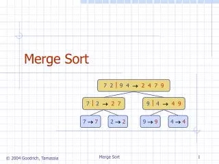
16. Mergesort Based on divide-and-conquer strategy • Divide the list into two smaller lists of about equal sizes • Sort each smaller list recursively • Merge the two sorted lists to get one sorted list

17. Mergesort • Divide-and-conquer strategy • recursively mergesort the first half and the second half • merge the two sorted halves together

18. see applet http://www.cosc.canterbury.ac.nz/people/mukundan/dsal/MSort.html

19. How do we divide the list? How much time needed? How do we merge the two sorted lists? How much time needed?

20. How to divide? • If an array A[0..N-1]: dividing takes O(1) time • we can represent a sublist by two integers left and right: to divide A[left..Right], we compute center=(left+right)/2 and obtain A[left..Center] and A[center+1..Right]

21. How to merge? • Input: two sorted array A and B • Output: an output sorted array C • Three counters: Actr, Bctr, and Cctr • initially set to the beginning of their respective arrays (1)   The smaller of A[Actr] and B[Bctr] is copied to the next entry in C, and the appropriate counters are advanced (2)   When either input list is exhausted, the remainder of the other list is copied to C

22. Example: Merge

23. Example: Merge... • Running time analysis: • Clearly, merge takes O(m1 + m2) where m1 and m2 are the sizes of the two sublists. • Space requirement: • merging two sorted lists requires linear extra memory • additional work to copy to the temporary array and back

25. Analysis of mergesort Let T(N) denote the worst-case running time of mergesort to sort N numbers. Assume that N is a power of 2. • Divide step: O(1) time • Conquer step: 2 T(N/2) time • Combine step: O(N) time Recurrence equation: T(1) = 1 T(N) = 2T(N/2) + N

26. Analysis: solving recurrence Since N=2k, we have k=log2 n

27. Don’t forget: We need an additional array for ‘merge’! So it’s not ‘in-place’!

28. Quicksort

29. Introduction • Fastest known sorting algorithm in practice • Average case: O(N log N) (we don’t prove it) • Worst case: O(N2) • But, the worst case seldom happens. • Another divide-and-conquer recursive algorithm, like mergesort

30. Quicksort • Divide step: • Pick any element (pivot) v in S • Partition S – {v} into two disjoint groups S1 = {x  S – {v} | x <=v} S2 = {x  S – {v} | x  v} • Conquer step: recursively sort S1 and S2 • Combine step: the sorted S1 (by the time returned from recursion), followed by v, followed by the sorted S2 (i.e., nothing extra needs to be done) S v v S1 S2 To simplify, we may assume that we don’t have repetitive elements, So to ignore the ‘equality’ case!

31. Example

33. Pseudo-code Input: an array a[left, right] QuickSort (a, left, right) { if (left < right) { pivot = Partition (a, left, right) Quicksort (a, left, pivot-1) Quicksort (a, pivot+1, right) } } Compare with MergeSort: MergeSort (a, left, right) { if (left < right) { mid = divide (a, left, right) MergeSort (a, left, mid-1) MergeSort (a, mid+1, right) merge(a, left, mid+1, right) } }

34. Two key steps • How to pick a pivot? • How to partition?

35. Pick a pivot • Use the first element as pivot • if the input is random, ok • if the input is presorted (or in reverse order) • all the elements go into S2 (or S1) • this happens consistently throughout the recursive calls • Results in O(n2) behavior (Analyze this case later) • Choose the pivot randomly • generally safe • random number generation can be expensive

36. In-place Partition • If use additional array (not in-place) like MergeSort • Straightforward to code like MergeSort (write it down!) • Inefficient! • Many ways to implement • Even the slightest deviations may cause surprisingly bad results. • Not stable as it does not preserve the ordering of the identical keys. • Hard to write correctly 

37. An easy version of in-place partition to understand, but not the original form int partition(a, left, right, pivotIndex) { pivotValue = a[pivotIndex]; swap(a[pivotIndex], a[right]); // Move pivot to end // move all smaller (than pivotValue) to the begining storeIndex = left; for (i from left to right) { if a[i] < pivotValue swap(a[storeIndex], a[i]); storeIndex = storeIndex + 1 ; } swap(a[right], a[storeIndex]); // Move pivot to its final place return storeIndex; } Look at Wikipedia

38. quicksort(a,left,right) { if (right>left) { pivotIndex = left; select a pivot value a[pivotIndex]; pivotNewIndex=partition(a,left,right,pivotIndex); quicksort(a,left,pivotNewIndex-1); quicksort(a,pivotNewIndex+1,right); } }

39. 19 6 j i A better partition • Want to partition an array A[left .. right] • First, get the pivot element out of the way by swapping it with the last element. (Swap pivot and A[right]) • Let i start at the first element and j start at the next-to-last element (i = left, j = right – 1) swap 6 5 6 4 3 12 19 5 6 4 3 12 pivot

40. 19 19 6 6 5 6 4 3 12 5 6 4 3 12 j j j i i i • Want to have • A[x] <= pivot, for x < i • A[x] >= pivot, for x > j • When i < j • Move i right, skipping over elements smaller than the pivot • Move j left, skipping over elements greater than the pivot • When both i and j have stopped • A[i] >= pivot • A[j] <= pivot <= pivot >= pivot

41. 19 19 6 6 j j i i • When i and j have stopped and i is to the left of j • Swap A[i] and A[j] • The large element is pushed to the right and the small element is pushed to the left • After swapping • A[i] <= pivot • A[j] >= pivot • Repeat the process until i and j cross swap 5 6 4 3 12 5 3 4 6 12

42. 19 19 19 6 6 6 j j j i i i • When i and j have crossed • Swap A[i] and pivot • Result: • A[x] <= pivot, for x < i • A[x] >= pivot, for x > i 5 3 4 6 12 5 3 4 6 12 5 3 4 6 12

43. Implementation (put the pivot on the leftmost instead of rightmost) void quickSort(int array[], int start, int end) { int i = start; // index of left-to-right scan int k = end; // index of right-to-left scan if (end - start >= 1) // check that there are at least two elements to sort { int pivot = array[start]; // set the pivot as the first element in the partition while (k > i) // while the scan indices from left and right have not met, { while (array[i] <= pivot && i <= end && k > i) // from the left, look for the first i++; // element greater than the pivot while (array[k] > pivot && k >= start && k >= i) // from the right, look for the first k--; // element not greater than the pivot if (k > i) // if the left seekindex is still smaller than swap(array, i, k); // the right index, // swap the corresponding elements } swap(array, start, k); // after the indices have crossed, // swap the last element in // the left partition with the pivot quickSort(array, start, k - 1); // quicksort the left partition quickSort(array, k + 1, end); // quicksort the right partition } else // if there is only one element in the partition, do not do any sorting { return; // the array is sorted, so exit } } Adapted from http://www.mycsresource.net/articles/programming/sorting_algos/quicksort/

44. void quickSort(int array[]) // pre: array is full, all elements are non-null integers // post: the array is sorted in ascending order { quickSort(array, 0, array.length - 1); // quicksort all the elements in the array } void quickSort(int array[], int start, int end) { … } void swap(int array[], int index1, int index2) {…} // pre: array is full and index1, index2 < array.length // post: the values at indices 1 and 2 have been swapped

45. With duplicate elements … • Partitioning so far defined is ambiguous for duplicate elements (the equality is included for both sets) • Its ‘randomness’ makes a ‘balanced’ distribution of duplicate elements • When all elements are identical: • both i and j stop  many swaps • but cross in the middle, partition is balanced (so it’s n log n)

46. A better Pivot Use the median of the array • Partitioning always cuts the array into roughly half • An optimal quicksort (O(N log N)) • However, hard to find the exact median (chicken-egg?) • e.g., sort an array to pick the value in the middle • Approximation to the exact median: …

47. Median of three • We will use median of three • Compare just three elements: the leftmost, rightmost and center • Swap these elements if necessary so that • A[left] = Smallest • A[right] = Largest • A[center] = Median of three • Pick A[center] as the pivot • Swap A[center] and A[right – 1] so that pivot is at second last position (why?) median3

48. 6 6 13 13 13 13 5 5 2 6 2 2 5 2 6 5 pivot pivot 19 A[left] = 2, A[center] = 13, A[right] = 6 6 4 3 12 19 Swap A[center] and A[right] 6 4 3 12 19 6 4 3 12 19 Choose A[center] as pivot Swap pivot and A[right – 1] 6 4 3 12 Note we only need to partition A[left + 1, …, right – 2]. Why?

49. Works only if pivot is picked as median-of-three. • A[left] <= pivot and A[right] >= pivot • Thus, only need to partition A[left + 1, …, right – 2] • j will not run past the beginning • because a[left] <= pivot • i will not run past the end • because a[right-1] = pivot The coding style is efficient, but hard to read 

50. i=left; j=right-1; while (1) { do i=i+1; while (a[i] < pivot); do j=j-1; while (pivot < a[j]); if (i<j) swap(a[i],a[j]); else break; }