Download
1 / 85
1.84k likes | 3.25k Views
SPREADSHEETS. MS EXCEL 2007. OBJECTIVE. You should be able to: State what is a spreadsheet Give applications of Spreadsheets State the components of a spreadsheet Navigate a spreadsheet. What is a Spreadsheet?.

E N D
SPREADSHEETS MS EXCEL 2007
OBJECTIVE • You should be able to: • State what is a spreadsheet • Give applications of Spreadsheets • State the components of a spreadsheet • Navigate a spreadsheet
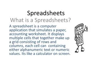
What is a Spreadsheet? A spreadsheet package is an application package that allows you to perform numeric calculations quickly and accurately.
USE OF SPREADSHEETS • PAYROLLS • KEEPING ACCOUNTS • PREPARING END OF TERM SCHOOL REPORTS • STOCK KEEPING • LOAN CALCULATION • FINANCIAL PLANS
COMPONENTS OF A SPREADSHEET • Each workbook contains three worksheets by default. • The worksheet window contains a grid of columns and rows. Columns are labeled alphabetically and rows are labeled numerically. • The intersection of a column and a row is a cell. • Cells can contain text, numbers or formulas. They are identified by their cell address/cell reference, which is the coordinates of an intersecting column and row, (example: A1, B12, etc.)
The cell pointer is a dark rectangle that highlights the cell you are working in (known as the Active cell). • The formula bar allows you to enter or edit data in the worksheet.
Labels, Values, Formula, Ranges • Labels are used to identify the data in the rows and columns of a worksheet. They also make your worksheet more readable and understandable. Labels can contain text and numerical data not used in calculations, such as dates times and address. • A Value is a piece of data that can be used in a calculation. A formula is an instruction to perform operations on values. A formula in Excel starts with an equal sign (=). E.g. =SUM(A2:A4) • A Range can be a cell or a group of adjoining cells treated as a unit. Example of a range: A2:A6 N.B. If a cell contains text and numbers and is not a formula, it is considered a label.
ACTIVITY 1 • Label the Excel Window
DEFAULT OPTIONS • There are 3 worksheets by default in a workbook • Text is automatically left aligned • Numbers are automatically right aligned
ACTIVITY 2 • Do Activity 1 on Pg 265 (purple bk.) or Pg 195 (blue bk.) • Use the navigating options to navigate your worksheet (see Pg 264:purple bk. or 194- blue bk.) • Save the Activity as ‘Sales’
HOME-WORK • READ Chapter 13 Pgs. 260-265. Do Exercise 1 on Page 266 (Log On to IT for CSEC- 2nd Edition)- Purple Book OR Chapter 11 Pgs. 192-196. Do Exercise 1 on Page 196- Blue book • DO Activity 1 on Pg 265 (Purple) or Pg 195 (Blue ) • Review Secondary Storage for Test next Day!
AFL: WHO AM I???? • I CAN BE USED IN A FORMULA AND WHEN ENTERED I AM RIGHT ALIGNED. • I AM VERTICAL IN A SPREADSHEET & I AM IDENTIFIED BY A LETTER. • I CANNOT BE USED IN A FORMULA AND I AM LEFT ALIGNED WHEN ENTERED. • B3:F9 IS KNOWN AS A ___________ • I AM HORIZONTAL & I AM IDENTIFIED BY A NUMBER • I AM FORMED BY THE INTERSECTION OF A ROW & COLUMN • THERE ARE THREE OF ME IN A WORKBOOK BY DEFAULT • I BEGIN WITH AN EQUAL SIGN • I AM USED TO PERFORM MATHEMATICAL CALULATIONS & PRODUCE GRAPHICAL DATA. • I AM USED TO IDENTIFY A CELL(E.G. A1)
REFERENCE SITES • http://www.lottieferguson.com/Excel_2003.pdf • http://edutech.msu.edu/online/Excel/ExcelIntro.html
LESSON 2- OBJECTIVES: At the end of the session you should be able to: • Use the formatting features: Bold, italic, underline, font, font size, borders, etc. • Use Alignment features: left, right, center align, Merge and Center • Change the orientation of text • Use the number formats • Edit the spreadsheet (cut, copy, paste) • Insert and delete a column and a row in the spreadsheet
KEY WORDS • Alignment • Format • Edit • Orientation
ACTIVITIES • ACTIVITY 1: • Go to http://www.teacherxpress.com/f.php?gid=35&id=20 (ii) Click on the Quiz Maker tab • Click on Dunkin Teacher • Choose Unit 7.4 • ACTIVITY 2: Create the spreadsheet and answer the questions given by the teacher.
HOME-WORK • Read Chapter 11 (Blue Book)- up to Pg 201/ Chapter 13 (Purple Book)- Page 267-272. Do Exercise 2, ques. 1 & 2 on Pg 202/Pg 273. • Write the steps of the tasks that had to be performed in the class activity. • Use text book and the online tutorial (Video Tutorials- MS Excel 2007: http://www.teacherxpress.com/f.php?gid=35&id=20to review steps and make notes
Example of writing steps: • Merge and Center the heading ‘PAYROLL’: (i) Select the range of cells A1:G1 by highlighting them (ii) Go to the Home ribbon (iii) Select the Alignment tab (iv) Click on Merge & Center
Using the Online Tutorial • Go to http://www.teacherxpress.com/f.php?gid=35&id=20 • Choose the Video Tutorialstab • Select Excel 2007 from the options listed on the left hand side of the web page. • Choose desired tutorial (by topic)
TERM 2: FORMULA & FUNCTIONS OBJECTIVES: At the end of these sessions you should be able to: • Formulate basic and more complex formulae • Use some pre-defined functions in Excel • Explain the difference between relative and absolute cell referencing
IMPORTANT!!!! • PLEASE NOTE: THE REFERENCES AND HOME-WORK ARE GIVEN FROM THE PURPLE TEXT BOOK. IF YOU ARE NOT SURE OF THE PAGES IN THE BLUE BOOK ASK YOUR TEACHER FOR THE EQUIVALENT REFERENCE!
Formulae in MS Excel • Electronic Spreadsheets allow you to perform calculations on data entered into the spreadsheet. • You can use an Excel 2007 formula for basic calculations, such as addition or subtraction, as well as more complex calculations. • In addition, if you change the data Excel will automatically recalculatethe answer without you having to re-enter the formula.
Use of Mathematical Operators The mathematical operators used in Excel formulae are: • Subtraction - minus sign ( - ) • Addition - plus sign ( + ) • Division - forward slash ( / ) • Multiplication – asterisk ( * ) • Exponentiation - caret ( ^ ) To create a formula in Excel you type an equal sign and combine the cell references of your data with the correct mathematical operator. (Read Pages 273-274 : Log On to IT for CSEC (2nd Ed.)
Order of Operators If more than one operator is used in a formula, there is a specific order that Excel will follow to perform these mathematical operations. This order of operations can be changed by adding brackets/parentheses to the equation. An easy way to remember the order of operations is to use the acronym BEDMAS (no not BODMAS) • The Order of Operations is: BracketsExponentsDivisionMultiplicationAdditionSubtraction
Order of Operations • Any operation(s) contained in brackets will be carried out first followed by any exponents. • After that, Excel considers division or multiplication operations to be of equal importance, and carries out these operations in the order they occur left to right in the equation. • The same goes for the next two operations – addition and subtraction. They are considered equal in the order of operations. Which ever one appears first in an equation, either addition or subtraction, is the operation carried out first.
The example shows how to add two numbers. The formula will add the numbers 3 + 2. STEPS:1. Type a 3 in cell E1 2. Type a 2 in cell E2 3. Type the = sign in cell E3 Simple Formula 4. Click on cell E1 with the mouse pointer to enter the cell reference into the formula.5. Type a plus ( + ) sign. 6. Click on cell E2 with the mouse pointer to enter the cell reference into the formula.7. Press the ENTER key on the keyboard. 8. The answer 5 should appear in cell E3. The formula in the formula bar will be =E1+E2
ACTIVITY 1 Perform the following calculations on the data in your spreadsheet: • Addition • Subtraction • Multiplication • Division • Exponentiation (see Fig. 1) • Your spreadsheet should look like Fig. 2. Fig. 1 Fig. 2
AFL • What is Automatic recalculation (w.r.t. using Excel)? • What is the order of precedence of the mathematical operators used in Excel? • Write the formula to add 2 numbers stored in cells A1 and A2 respectively.
Using a more complex formula ACTIVITY 2: The activity is a Marksheet that calculates the Total Marks the students attained and their Average Mark: STEPS: • Enter the data as seen in the spreadsheet (SEE next slide). • Enter the formula in cell F4 (=C4+D4+E4) • Copy and paste the formula to cells F5:F8 • Enter the formula G4 (=F4/300)*100 • Copy and paste the formula to cells G5:G8
HOME-WORK • Do Activity 4 and Exercise 3- Page 274- 275 (Log On to IT for CSEC- 2nd Ed.)
FUNCTIONS Excel uses Functions (which are mathematical expressions already available in Excel) and formulae ( mathematical expressions that you create) to dynamically create results from data in your worksheet. Each of Excel’s Functions is a predefined formula acting on a range of cells that you select. The range of cells in the function that is selected is referred to as an argument.
FUNCTIONS • The following functions will be looked at in our class: • SUM • COUNT • MAX • MIN • AVERAGE • (Read Page 276-278 (Ch 13): Log On to IT for CSEC (2nd Edition)
We said earlier if you wanted to add a series of numbers you would enter an equal sign followed by the cells you want Excel to add up. Example: = B4 + B5 + B6 + B7 • But this is not a good way to add up in Excel. It could get very tedious if you had to type out say 100 cell references by hand. The easy way is to get Excel to do the work for you. That's where SUM comes in!!
Example using SUM • Consider the following example in the next slide. We want to find the total sales for Monday, Tuesday, Wednesday, etc. • First you type an equal sign, the word SUM then open brackets) in cell B8. • Then you highlight the range of cells with the data you want to be added. In this case, B4:B7. • Then you enter the closed brackets and press enter
You can copy and paste the formula to the other cells to get the totals for the other days instead of retyping the formula.
Now do the Activity for yourself. • After you have completed the activity, click on cells B8, C8, D8, E8 and F8 and write the formula in your books. What is your observation?
If you noticed that the cell ranges changed with respect to the new location of the formula then YOU ARE RIGHT!! B8’s formula is =SUM (B4:B7) C8’s formula is =SUM (C4:C7) D8’s formula is =SUM (D4:D7) E8’s formula is =SUM (E4:E7) and so on. This is known as relative cell referencing!!!!
AVERAGE FUNCTION First, what is in an average? In math, an average is a number derived by dividing how many there are in a list by the list total. For example, suppose a list of student scores in an exam was this: 9, 7, 6, 7, 8, 4, 3, 9. We only have eight scores. To get the average score we first need to get the total. So add up the numbers in the list: 9 + 7 + 6 + 7 + 8 + 4 + 3 + 9 = 53. Next divide by how many there are in the list: 8. So to get the average score the sum is 53 divided by 8. The answer is 6.625. Which means that the average score in the exam was 6.625.
In Excel there is a predefined function to determine the average, known as AVERAGE. Using the previous example, let’s find the average amount of chocolates that are sold each day. Again, we start with an equal sign, followed by the function, then the range in brackets. Press enter. The result should be:16.5 (format your number to 0 decimal places to get 17). Copy and paste the formula to the other cells.
MAX AND MIN FUNCTIONS The MAX function allows you to find the largest value amongst a list of values. The MIN function allows you to find the smallest value amongst a list of values. Using the same activity as before, let’s find the largest amount of chocolates sold each day and the least amount of chocolates sold each day!