Download
1 / 1
10 likes | 120 Views
Skill Assessment of Multiple Hypoxia Models in the Chesapeake Bay and Implications for Management Decisions. Isaac (Ike) Irby 1 , Marjorie Friedrichs 1 , Yang Feng 1 , Raleigh Hood 2 , Jeremy Testa 2 , Carl Friedrichs 1

E N D
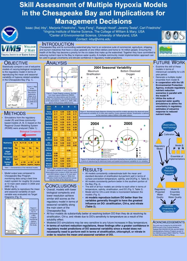
Skill Assessment of Multiple Hypoxia Models in the Chesapeake Bay and Implications for Management Decisions Isaac (Ike) Irby1, Marjorie Friedrichs1, Yang Feng1, Raleigh Hood2, Jeremy Testa2, Carl Friedrichs1 1Virginia Institute of Marine Science, The College of William & Mary, USA 2Center of Environmental Science, University of Maryland, USA Contact: iirby@vims.edu Introduction Chesapeake Bay and its surrounding watershed play host to an extensive suite of commercial, agriculture, shipping, and tourism industries that have a value upwards of one trillion dollars and home to 16 million people. Ensuring the health of the Bay has become a priority for the six states that make up the watershed. Together they have committed to reducing nutrient input to the Bay to improve water quality. A multiple community model implementation approach can be used to gauge uncertainty and elevate confidence in regulatory model projections. Observations and Forcings Future Work Objective Analysis • Examine the skill of these models in terms of interannual variability for a 25 year period. • Generate a multiple model ensemble from model B. • In cooperation with the US Environmental Protection Agency, evaluate regulatory nutrient reduction scenarios in parallel with the model R • Utilize the suite of projected water quality simulations to define the uncertainty in regulatory estimates of estuarine response to reduced nutrient loads. Statistically compare a set of estuarine models of varying biological complexity to the regulatory model in terms of reproducing the mean and seasonal variability of hypoxia related variables in the Chesapeake Bay (Fig. 1). 2004 Seasonal Variability Bottom Dissolved Oxygen Maximum Stratification Calibration Figure 2. Location of the 10 Chesapeake Bay Program monitoring stations utilized in the study. R A R A Model B Regulatory Model Figure 3. Target Diagram analysis: the total root mean square difference (RMSD) between the observations and the model results, normalized by the standard deviation of the observations. (Jolliff et al., 2009, JMS, doi10.1016/j.jmarsys.2008.05.014). C B C B C Ensemble of Implementations Biological Complexity Methods Figure 4. Normalized target diagrams showing how well the models reproduce the observed mean and seasonal variability at 10 main stem stations. Colors represent latitude. Stratification is defined as the maximum value of dS/dz in the water column. Nutrient Reduction Scenario • Simulations from the regulatory model (R) and three community-based models (A, B, C) based on the Regional Ocean Modeling System (ROMS) were analyzed (Table 1): • Model output was compared to Chesapeake Bay Program monitoring data using a best time match system for roughly 34 cruises at 10 main stem station in 2004 and 2005 (Fig. 2). • Model ability to reproduce the mean and seasonal variability of each variable was evaluated via Target Diagrams (Fig. 3). 2005 2004 Table 1. Characteristics of the individual models. Regulatory Projected Water Quality Model B Ensemble Projected Water Quality R A B C Estimate Uncertainty in Projections Figure 5. Normalized target diagrams for 2004/2005 illustrating how well the four models perform in terms of reproducing the observed means and spatial and seasonal variability for six variables. Figure 1. Map of the Chesapeake Bay and its watershed. (Najjaret al., 2010, ECSS, doi10.1016/j.ecss.2009.09.026). Results Table 2. Total normalized RMSD computed for multiple variables of each model using observations from cruises in 2004 (top value) and 2005 (bottom value) at 10 main stem stations shown in Figure 2. White font indicates model results that perform worse than the mean of the observations. • All models consistently underestimate both the mean and standard deviation of stratification but perform well in terms of surface and bottom temperature, salinity, and DO(Fig. 4, Table 2). • All models consistently perform better in the southern portion of the Bay (Fig. 4). • The skill of all four models are similar to each other in terms of temperature, salinity, stratification, and DO (Fig. 5, Table 2). • Model skill for Chl-a and nitrate is inconsistent between the models (Fig. 5). • All models reproduce bottom DO better than the variables generally thought to have the greatest influence on DO: stratification, Chl-a, and nitrate (Table 2). Conclusions • Overall, models with lower biological complexity and lower resolution achieve similar skill scores as the regulatory model in terms of seasonal variability along the main stem of the Chesapeake Bay. • All four models do substantially better at resolving bottom DO than they do at resolving its stratification, Chl-a, and nitrate due to DO’s sensitivity to temperature as a result of the solubility effect. • Modeled DO simulations may be very sensitive to any future increases in Bay temperature. • In terms of nutrient reduction regulations, these findings offer a greater confidence in regulatory model predictions of DO seasonal variability since a model does not necessarily need to perform well in terms of stratification, chlorophyll, or nitrate in order to resolve the mean and seasonal variation of DO. Acknowledgements This work was funded by the NOAA NOS IOOS as part of the Coastal Modeling Testbed (NA13NOS0120139) and the NASA Interdisciplinary Science Program as part of the USECoS project (NNX11AD47G). Thanks to Aaron Bever and Ping Wang.