Download
1 / 33
350 likes | 480 Views
High order explicit methods for parabolic equations and stiff ODEs (DUMKA3, DUMKA4, ROCK2, ROCK4). Alexei Medovikov Tulane University. A. Abdulle, A. Medovikov Second order Chebyshev methods based on orthogonal polynomials. Numerische Mathematik V90.1. pp.1-18

E N D
High order explicit methods for parabolic equationsand stiff ODEs(DUMKA3, DUMKA4, ROCK2, ROCK4) Alexei Medovikov Tulane University A. Abdulle, A. Medovikov Second order Chebyshev methods based on orthogonal polynomials. Numerische Mathematik V90.1. pp.1-18 Medovikov A.A. High order explicit methods for parabolic equations. BIT, V38,No2,pp.372-390 Lebedev V.I., Medovikov A.A. Method of second order accuracy with variable time steps. Izv. Vyssh. Uchebn. Zaved. Mat. no. 9, 52--60 (English translation).
WELCOME TO DUMKALAND Explicit numerical methods for stiff differential equations DUMKA3 - integrates initial value problems for systems of first order ordinary differential equations y'=f(y,t). It is based on a family of explicit Runge-Kutta-Chebyshev formulas of order three. It uses optimal third order accuracy stability polynomials with the largest stability region along the negative real axis.
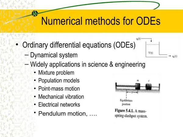
Examples of solution of stiff differential equations by explicit methods Brusselator equation Nagumo nerve conduction equation Burgers equation
Summary • Stability: Explicit methods have small stepsize , due to conditional stability • Variable steps can be used to maximize mean stepsize of a sequence of explicit methods • Optimal sequence of explicit steps can be found in terms of roots of stability polynomials, which approximate exponential function and possess Chebyshev alternation • Asymptotic formulas and orthogonal polynomials can be used to construct such polynomials, even very high degree polynomials (n > 1000) • Accuracy: In order to construct high order explicit methods for non-linear ODE, we start with stability polynomials and we use B-series in order to satisfy order conditions, and build Runge-Kutta methods for non-liner ODEs • Efficient stepsize control and step rejection procedure are achieved via embedded methods • For automatic computation of spectral radius we used non-linear power method.
Stability analysis of explicit RK methods ODEs: Explicit Euler method: Test equation: Stability function: where is a total step Stability region: Goal: Find stability polynomial which maximize average stepsize , given
Stability analysis of explicit RK methods Explicit Euler method: Stability condition of explicit Euler method: Linear stability analysis for non-linear ODEs: where Linear stability RK methods vs. Stability RK methods?
Can we solve stiff ordinary differential equations (ODE) by explicit methods with stepsize larger than 2/M?Example: Consider two steps and where
Original idea of Runge-Kutta-Chebyshev methods Consider sequence of Euler steps and find an optimal polynomial as large as possible If we have found the optimal stability polynomial, the variable sequence of steps can be found in terms of the roots of the stability polynomial
The solution for n-stage Runge-Kutta-Chebyshev method order p=1 is given by Chebyshev stability polynomial.
Theorem (T. Riha): Among all polynomials of the order p the polynomial which possess Chebyshev alternant, would maximize real stability interval or equivalently, the polynomial which possess Chebyshev alternant: has maximal possible stepsize , given stability
Two algorithms of computation of stability polynomials: • For given n calculate weight • and roots via asymptotic formula for polynomials • of the least deviation from zero: • so that the polynomial satisfies (1), • 2. For given n calculate weight • so that the polynomial satisfies (1), • where is orthogonal polynomial with the weight DUMKA3,4 ROCK2,4, RKC
Accuracy:Order conditions of Runge-Kutta methods Taylor expansions of the exact solution and numerical solution : where
Construction of pth order composition method Let us consider two consecutive steps by Runge-Kutta methods A and B. We call the method which is the result of one step of A and one step of B as the composition method C=B(A) Stability function of the composition method C is the product of stability functions of the methods A and B Theory of composition methods allows to calculate Taylor expansion of composition methods:
Given method A, define method B such that method C=B(A) will be method of the order p and stability function of the method C will be product of the stability functions of the methods A and B. Coefficients of Taylor expansion of the method B can be expressed in terms of coefficients of the methods C and B