Download
1 / 54
580 likes | 1.16k Views
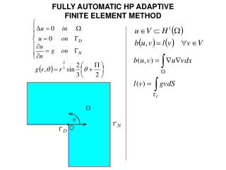
Field equations and The Finite Element Method (FEM). TBME08 Johannes Johansson. Field equations. With the circuit approach we have used discrete components (objects) to model systems. What if we are interested in the behavior of some property in different parts of a component?. V 1. -. -.

E N D
Field equations and The Finite Element Method (FEM) TBME08 Johannes Johansson
Field equations • With the circuit approach we have used discrete components (objects) to model systems. • What if we are interested in the behavior of some property in different parts of a component? V1 - - - a E=? + + V2 +
Scalar fields (rank 0 tensors) Scalar quantities are described by single values at each point in space and time. In cartesian coordinates: V = V(x,y,z,t) Scalar variables are usually denoted in italic.
Examples of scalar quantities Temperature: Altitude: Pressure: Electric potential:
Vector fields (rank 1 tensors) Vector quantities are described by vectors at each point in space and time. In cartesian coordinates: Vector variables are usually denoted in bold italic.
Examples of vector quantities Flow velocity: Electric current: Force:
Tensor fields (rank 2 tensors) (Rank 2) tensor quantities are described by an matrix at each point in space and time. Tensors are difficult to visualise
Examples of tensor quantities Stress and strain tensors in deformations: Diffusion tensors:
Nabla operator, Cartesian coordinates: Laplacian:
Gradient The gradient describes the slope of a field. It will increase the rank of the field, e.g. the gradient of a scalar field is a vector field and the gradient of a vector field is a (2nd rank) tensor field.
Gradient, example Assume a scalar field V described by V = x + y The gradient is then
Divergence Scalar product between the nabla operator and the field quantity: The divergence describes sources and sinks in a field. It will decrease the rank of the field, e.g. the divergence of a vector field is a scalar field and the divergence of a (2nd rank) tensor field is a vector field.
Positive divergence Assume a vector field A described by The divergence is then
Negative divergence Assume a vector field A described by The divergence is then
Curl Vector product between the nabla operator and the field quantity: The curl describes angular moments in a field. It does not change the rank of the field.
Positive curl = clockwise Assume a vector field A described by The curl is then
Negative curl = counterclockwise Assume a vector field A described by The curl is then
Vortexes are not required for curl Assume a vector field A described by The curl is then
Example: Laplace’s equation Commonly used to describe fields in homogeneous and isotropic media, e.g. electric fields in free space.
The Finite Element Method (FEM) • Analytical solutions for field equations only exist for some special cases with simple geometries. For other cases some numerical approach is needed. • A popular method is the finite element method where the geometrical model is divided in many small elements. V1 Example: Two plates with different charge. - - - a E=? + + V2 +
FEM: Choose appropriate mathematical model E.g. electrostatics: FEM software usually have pre-defined mathematical models to choose from.
FEM: Create a geometrical model CAD is used to draw an appropriate geometry. In the example here the distance between the plates, a, is 2 mm.
FEM: Assign material parameters The geometrical model consist of subdomains.
FEM: Assign boundary conditions Ground (V = 0V) Zero charge Axis of symmetry V = 1 V
FEM: Generate mesh • The mathematical model is approximated with polynomials of different order over each element. • Higher order elements give more accurate solutions but are more taxing on computer power. • States are calculated in each node (can yield very large state matrices, especially in 3D). Nodes Element
FEM: Check of the solution is reasonable Compare the results with measurements or known analytical solutions.
FEM: Refine mesh • Higher mesh density gives more accurate solution but is more taxing on the computer • Start with a coarse mesh and then refine it
Symmetry • Three-dimensional field calculations are usually very taxing on computer resources. • If the geometric dimension of the model can be reduced calculations will be much faster and require much less memory.
Translational symmetry V(x,y,z)V(x,y) Model Modelled area No or small changes in this direction Long object
Improper use of translational symmetry Modelled area Model Considerable variations in this direction What really is modelled here
Axial symmetry Cylindrical coordinates: V(x,y,z)V(r,z) Modelled area Axially symmetric object Model Axis of symmetry
Improper use of axial symmetry Model What really is modelled here Objects
Homogeneity - heterogeneity • A homogeneous domain has the same characteristics everywhere in space. • The characteristics of a heterogeneous domain varies in space. • Whether a domain should be considered homogeneous or heterogeneous usually depends on the scale of interest.
Isotropy - anisotropy • An isotropic domain has the same characteristics in all directions for any given point. • The characteristics are different in different directions for an anisotropic domain.
Examples of anisotropic matter • Muscles • White brain matter • Polarisation filters Poor electric conductivity - electromagnetic waves pass through Good electric conductivity - electromagnetic waves are absorbed or reflected
Example: Steady state electric currents State variable: Electric potential, V, (V) J = electric current density (A/m2) E = electric field (V/m) = electric conductivity (S/m)
Example: Steady state electric currents • In a homogeneous and isotropic media this equation reduces to Laplace’s equation (which has made many to mix up the equations). • The electric conductivity is a scalar quantity for isotropic media and a (2nd rank) tensor quantity for anisotropic media. (Assumed to be scalar in last slide.) • Compare with Kirchoff’s current law:
Electric currents in biological tissue Cell membrane (thin electric insulator) proteins • The cell membrane blocks direct currents but allow for capacitive alternating currents. • The heterogeneous cell structure is modelled as homogeneous tissue with a frequency-dependent electric conductivity. - - salt ions + + + - intracellular fluid extracellular fluid
Simulation of electric field around DBS electrode • Electric pulses are used to jam overactive neural structures in the brain • Here the electric field intensity is simulated and presented as isosurfaces
Example: Heat transfer State variable:Temperature, T, (K or °C) Heat source (or sink) Convective heat transfer Temperature change Conductive heat transfer = Mass density (kg/m3) c = Specific heat capacity (J/(kgK)) u= Velocity (m/s) k = Thermal conductivity (W/(mK))
Example: Resistive (Joule) heating Compare with: P = IU (W)
Radio frequency (RF) ablation • A temperature-controlled current is used to kill overactive tissue. The proteins of tissue coagulate at about 50-60 °C. The proteins stick together, which causes the tissue to become whiter (higher light scattering) and stiffer. Bonds in the proteins break. Bonds form between the proteins.
RF ablation The heating is focussed to the tissue closest to the electrode tip. The heat then spreads outwards and inwards. (˚C) (W/m3)
Example: Navier-Stokes equations State variables: Pressure, p, (N/m2) Velocity, u, (m/s) Viscous friction force Fluid inertia Gravity force Pressure gradient Incompressible fluid = Dynamic viscosity (Ns/m2) g = Acceleration of gravity (m/s2)
Aterosclerotic blood vessel • Model of a blood vessel with a radius of 1 mm and an average flow velocity of 0.1 m/s. • A constriction increases the resistance to flow and thus the pressure required to maintain a certain flow speed.
Compare with Poiseuille’s formula for stationary flow through a straight tube v = Velocity in the axial direction (m/s) l = Tube length (m) R = Tube radius (m) r = Radial coordinate (m)
Saline-enhanced RF ablation • When killing tumours a large volume of tissue destruction is usually desired • Salt water can be used to enhance the heat transport through higher electric conductivity in combination with fluid flow.