Linear Models I

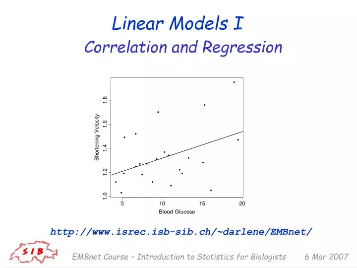
1. Linear Models I http://www.isrec.isb-sib.ch/~darlene/EMBnet/ Correlation and Regression EMBnet Course – Introduction to Statistics for Biologists

2. Univariate Data (Review) • Measurements on a singlevariable X • Consider a continuous(numerical)variable • Summarizing X • Numerically • Center • Spread • Graphically • Boxplot • Histogram EMBnet Course – Introduction to Statistics for Biologists

3. Bivariate Data • Bivariate data are just what they sound like – data with measurements on two variables; let’s call them Xand Y • Here, we are looking at two continuousvariables • Want to explore the relationship between the two variables • Can also look for association between two discrete variables; we won’t cover that here EMBnet Course – Introduction to Statistics for Biologists

4. Scatterplot • We can graphically summarize a bivariate data set with a scatterplot (also sometimes called a scatter diagram) • Plots values of one variable on the horizontal axis and values of the other on the vertical axis • Can be used to see how values of 2 variables tend to move with each other (i.e. how the variables are associated) EMBnet Course – Introduction to Statistics for Biologists

5. Scatterplot: positive association EMBnet Course – Introduction to Statistics for Biologists

6. Scatterplot: negative association EMBnet Course – Introduction to Statistics for Biologists

7. Scatterplot: real data example EMBnet Course – Introduction to Statistics for Biologists

8. Numerical Summary • Typically, a bivariate data set is summarized numerically with 5 summary statistics • These provide a fair summary for scatterplots with the same general shape as we just saw, like an oval or an ellipse • We can summarize each variable separately : Xmean, XSD; Ymean, YSD • But these numbers don’t tell us how the values of X and Yvary together EMBnet Course – Introduction to Statistics for Biologists

9. Correlation Coefficient • The (sample) correlation coefficientr is defined as the average value of the product (Xin SUs)*(Y in SUs) • SU = standard units = (X – mean(X))/SD(X) • ris a unitless quantity • -1 r  1 • ris a measure of LINEAR ASSOCIATION EMBnet Course – Introduction to Statistics for Biologists

10. R:correlation • In R: > cor(x,y) • Note, however, that if there are missing values (NA), then you will get an error message • Elementary statistical functions in R require • no missing values, or • explicit statement of what to do with NA EMBnet Course – Introduction to Statistics for Biologists

11. R:NA in statistical functions • For single vector functions (e.g.mean, var, sd), give the argument na.rm=TRUE • For cor, though, there are more possibilities for dealing with NA • See the argument use and the methods given there: ?cor EMBnet Course – Introduction to Statistics for Biologists

12. What r is... • r is a measure of LINEAR ASSOCIATION • The closer r is to –1 or 1, the more tightly the points on the scatterplot are clustered around a line • The sign of r(+ or -) is the same as the sign of the slope of the line • When r= 0, the points are not LINEARLY ASSOCIATED– this does NOTmean there is NO ASSOCIATION EMBnet Course – Introduction to Statistics for Biologists

13. ...and what ris not • r is a measure of LINEAR ASSOCIATION • r does NOT tell us if Yis a function of X • rdoes NOT tell us if XcausesY • r does NOT tell us if YcausesX • r does NOTtell us what the scatterplot looks like EMBnet Course – Introduction to Statistics for Biologists

14. r 0: random scatter EMBnet Course – Introduction to Statistics for Biologists

15. r 0: curved relation EMBnet Course – Introduction to Statistics for Biologists

16. r  0: outliers outliers EMBnet Course – Introduction to Statistics for Biologists

17. r  0: parallel lines EMBnet Course – Introduction to Statistics for Biologists

18. r 0: different linear trends EMBnet Course – Introduction to Statistics for Biologists

19. Correlation is NOT causation • You cannot infer that since Xand Y are highly correlated (r close to –1 or 1) that X is causing a change in Y • Y could be causing X • X and Y could both be varying along with a third, possibly unknown factor (either causal or not; often ‘time’ ): • Polio and soft drinks: US polio cases tended to go up in summer, so do sales of soft drinks => does not mean that soft drinks cause polio EMBnet Course – Introduction to Statistics for Biologists

20. Predicting shortening velocity • Say we are interested in getting a value for shortening velocity (thuesen data) • We could measure it, but that may be difficult/expensive/impractical/etc. • If we have a measurement on a variable that is related to shortening velocity – such as blood glucose, say – then perhaps there would be some way to use that measurement to estimate or predict shortening velocity • What relation is suggested by the scatterplot? EMBnet Course – Introduction to Statistics for Biologists

21. SV vs. BG EMBnet Course – Introduction to Statistics for Biologists

22. (Simple) Linear Regression • Refers to drawing a (particular, special) line through a scatterplot • Used for 2 broad purposes: • Explanation • Prediction • Equation for a line to predict y knowing x (in slope-intercept form) looks like: y = a + b*x • a is called the intercept ; bis the slope EMBnet Course – Introduction to Statistics for Biologists

23. Which line? • There are many possible lines that could be drawn through the cloud of points in the scatterplot ... • How to choose? EMBnet Course – Introduction to Statistics for Biologists

24. Regression Prediction • The regression prediction says: when Xgoes up by 1 SD, predicted Y goes up **NOT by 1 SD**, but by only r SDs (down if ris negative) • This prediction can be expressed as a formula for a line in slope-intercept form: predicted y = intercept+ slope * x, with slope = r * SD(Y)/SD(X) intercept = mean(Y) – slope * mean(X) EMBnet Course – Introduction to Statistics for Biologists

25. Least Squares • Q: Where does this equation come from? A: It is the line that is ‘best’ in the sense that it minimizesthe sum of the squared errors in the vertical (Y) direction Y * * * errors * * X EMBnet Course – Introduction to Statistics for Biologists

26. Interpretation of parameters • The regression line has two parameters: the slope and the intercept • The regression slopeis the average change in Y when X increases by 1 unit • The intercept is the predicted value for Y when X = 0 • If the slope = 0, then Xdoes not help in predicting Y (linearly) EMBnet Course – Introduction to Statistics for Biologists

27. Another view of the regression line • We can divide the scatterplot into regions (X-strips) based on values of X • Within each X-strip, plot the average value of Y (using only Y values that have X values in the X-strip) • This is the graph of averages • The regression line can be thought of as a smoothed version of the graph of averages EMBnet Course – Introduction to Statistics for Biologists

28. Scatterplot (again) EMBnet Course – Introduction to Statistics for Biologists

29. Creating X-strips EMBnet Course – Introduction to Statistics for Biologists

30. Graph of averages EMBnet Course – Introduction to Statistics for Biologists

31. Residuals • There is an errorin making a regression prediction: error = observed Y – predicted Y • These errors are called residuals EMBnet Course – Introduction to Statistics for Biologists

32. Pitfalls in regression • ecological regression • when the units are aggregated, for example death rates from lung cancer vs. percentage of smokers in cities => relationship can look stronger than it actually is (we don’t know whether it is the smokers that are dying of lung cancer) • extrapolation • don’t know what the relationship between X and Y looks like outside the range of the data • regression effect/fallacy • test-retest and regression toward the mean EMBnet Course – Introduction to Statistics for Biologists

33. Modeling Overview • Want to capture important features of the relationship between a (set of) variable(s)and one or more response(s) • Many models are of the form g(Y) = f(x) + error • Differences in the form of g, f and distributional assumptions about the error term EMBnet Course – Introduction to Statistics for Biologists

34. Linear Modeling • A simple linear model: E(Y) = 0 + 1x • Gaussian measurement model: Y = 0 + 1x + , where  ~ N(0, 2) • More generally: Y = X + , where Y is n x 1, X is n x p,  is p x 1,  is n x 1, often assumed N(0, 2Inxn) EMBnet Course – Introduction to Statistics for Biologists

35. R:linear modeling with lm • To compute regression coefficients(intercept and slope(s)) in R: lm(y ~ x) • Can read ~ as ‘described (or modeled) by ’ • Example : to predict ventricular shortening velocity from blood glucose: > lm(short.velocity ~ blood.glucose) Call: lm(formula = short.velocity ~ blood.glucose) Coefficients: (Intercept) blood.glucose 1.09781 0.02196 EMBnet Course – Introduction to Statistics for Biologists

36. R:using lm • You can do much more complicated modeling with lm • The result of lm is a model object which contains additional information beyond what gets printed • To see some of these other quantities: > summary(lm(short.velocity ~ blood.glucose)) EMBnet Course – Introduction to Statistics for Biologists

37. R:summarizing lm > summary(lm(short.velocity~blood.glucose)) Call: lm(formula = short.velocity ~ blood.glucose) Residuals: Min 1Q Median 3Q Max -0.40141 -0.14760 -0.02202 0.03001 0.43490 Coefficients: Estimate Std. Error t value Pr(>|t|) (Intercept) 1.09781 0.11748 9.345 6.26e-09 *** blood.glucose 0.02196 0.01045 2.101 0.0479 * --- Signif. codes: 0 `***' 0.001 `**' 0.01 `*' 0.05 `.' 0.1 ` ' 1 Residual standard error: 0.2167 on 21 degrees of freedom Multiple R-Squared: 0.1737, Adjusted R-squared: 0.1343 F-statistic: 4.414 on 1 and 21 DF, p-value: 0.0479 EMBnet Course – Introduction to Statistics for Biologists

38. Basic model checking • Examination of residuals • Normality • Time effects • Nonconstant variance • Curvature • Detection of influential observations • Hat matrix • We will do a little of this in the practical EMBnet Course – Introduction to Statistics for Biologists

39. QQ-Plot • Quantile-quantile plot • Assess whether a sample follows a particular (e.g. normal) distribution (or to compare two samples) • A method for looking for outliers when data are mostly normal Sample Sample quantile is 0.125 Theoretical Value from Normal distribution which yields a quantile of 0.125 (= -1.15) EMBnet Course – Introduction to Statistics for Biologists

40. Typical deviations from straight line patterns • Outliers • Curvature at both ends (long or short tails) • Convex/concave curvature (asymmetry) • Horizontal segments, plateaus, gaps EMBnet Course – Introduction to Statistics for Biologists

41. Outliers EMBnet Course – Introduction to Statistics for Biologists

42. Long Tails EMBnet Course – Introduction to Statistics for Biologists

43. Short Tails EMBnet Course – Introduction to Statistics for Biologists

44. Asymmetry EMBnet Course – Introduction to Statistics for Biologists

45. Plateaus/Gaps EMBnet Course – Introduction to Statistics for Biologists

46. Hat values • High leverage points are far from the center, and have potentially greater influence • One way to assess points is through the hat values (obtained from the hat matrix H): ŷ = Xb = X(X’X)-1X’y = Hy hi = Σjhij2 • Average value of h = number of coefficients/n (including the intercept) = p/n • Cutoff typically 2p/n or 3p/n EMBnet Course – Introduction to Statistics for Biologists

47. CIs and hypothesis tests • With some assumptions about the error distribution, you can make confidence intervals or carry out hypothesis tests : • for the regression line • prediction interval for future observation • hypothesis tests for coefficients • We will not worry about the details of these EMBnet Course – Introduction to Statistics for Biologists