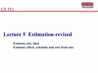
Download
1 / 39
390 likes | 571 Views
CS 551. Lecture 5 Estimation-revised Estimate size, then Estimate effort, schedule and cost from size. Project Metrics. Cost and schedule estimation Measure progress Calibrate models for future estimating Metric/Scope Manager Product Number of projects x number of metrics = 15-20.

E N D
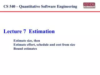
CS 551 Lecture 5 Estimation-revised Estimate size, then Estimate effort, schedule and cost from size
Project Metrics • Cost and schedule estimation • Measure progress • Calibrate models for future estimating • Metric/Scope Manager Product Number of projects x number of metrics = 15-20
Approaches to Cost Estimtation • By expert • By analogies • Decomposition • Parkinson’s Law; work expands to fill time available • Pricing to win: price is set at customer willingness to pay • Lines of Code • Function Points • Mathematical Models: Function Points & COCOMO
Boehm: “A project can not be done in less than 75% of theoretical time” Time Ttheoretical 75% * Ttheoretical Linear increase Staff-month Impossible design But, how can I estimate staff months? Ttheoretical = 2.5 * 3√staff-months
Sizing Software Projects • Effort = (productivity)-1 (size)c productivity ≡ staff-months/kloc size ≡ kloc Staff months 500 Lines of Code or Function Points
Understanding the equations Consider a transaction project of 38,000 lines of code, what is the shortest time it will take to develop? Module development is about 400 SLOC/staff month Effort = (productivity)-1 (size)c = (1/.400 KSLOC/SM) (38 KSLOC)1.02 = 2.5 (38)1.02 ≈ 100 SM Min time = .75 T= (.75)(2.5)(SM)1/3 ≈ 1.875(100)1/3 ≈ 1.875 x 4.63 ≈ 9 months
How many software engineers? • 1 full time staff week = 40 hours, 1 student week = 20 hours. • Therefore, our estimation of 100 staff months is actually 200 student months. • The period of coding is December 2004 through April 2005, which is a period of 5 months. • 200 staff months/5 months = 40 student software engineers, therefore simplification is mandatory As of 8Nov07
Productivity= f (size) Bell Laboratories data Capers Jones data Productivity (Function points / staff month) Function Points
Average Change Processing Time: for two Systems of Systems Average workdays to process changes Thanks to Barry Boehm
SW SW Effect of ignoring software structure • Software risks discovered too late • Slow, buggy change management (WBS-based) Software SW Thanks to Barry Boehm
Software Development Schedule TrendsNumber of Years ≈ 0.04 * cube root (NCKSLOC) SW Years to Develop Software,Hardware HW Thousands of source lines of code (KSLOC)
The Cone of Uncertainty: Usual result of total commitment Better to buy information to reduce risk ^ Inadequate PDR Thanks to Barry Boehm 05/22/2007 (c) USC-CSSE 12
There is Another Cone of Uncertainty:Shorter increments are better Uncertainties in competition, technology, organizations, mission priorities 05/22/2007 (c) USC-CSSE 13
The Incremental Commitment Life Cycle Process: Overview Stage I: Definition Stage II: Development and Operations Anchor Point Milestones Concurrently engr. Incr.N (ops), N+1 (devel), N+2 (arch) Concurrently engr. OpCon, rqts, arch, plans, prototypes
Increment View Thanks to Barry Boehm
RUP/ICM Anchor Points Enable Concurrent Engineering C V A D I O C C C C O C D R R R C R Thanks to Barry Boehm
Lines of Code • LOC ≡ Line of Code • KLOC ≡ Thousands of LOC • KSLOC ≡ Thousands of Source LOC • NCKSLOC ≡ New or Changed KSLOC
Bernstein’s rule of thumb Productivity per staff-month: • 50 NCSLOC for OS code (or real-time system) • 250-500 NCSLOC for intermediary applications (high risk, on-line) • 500-1000 NCSLOC for normal applications (low risk, on-line) • 10,000 – 20,000 NCSLOC for reused code Reuse note: Sometimes, reusing code that does not provide the exact functionality needed can be achieved by reformatting input/output. This decreases performance but dramatically shortens development time.
QSE Lambda Protocol • Prospectus • Measurable Operational Value • Prototyping or Modeling • sQFD • Schedule, Staffing, Quality Estimates • ICED-T • Trade-off Analysis
Heuristics for requirements engineering • Move some of the desired functionality into version 2 • Deliver product in stages 0.2, 0.4… • Eliminate features • Simplify Features • Reduce Gold Plating • Relax the specific feature specificaitons
Function Point (FP) Analysis • Useful during requirement phase • Substantial data supports the methodology • Software skills and project characteristics are accounted for in the Adjusted Function Points • FP is technology and project process dependent so that technology changes require recalibration of project models. • Converting Unadjusted FPs (UFP) to LOC for a specific language (technology) and then use a model such as COCOMO.
Function Point Calculations • Unadjusted Function Points UFP= 4I + 5O + 4E + 10L + 7F, Where I ≡ Count of input types that are user inputs and change data structures. O ≡ Count of output types E ≡ Count of inquiry types or inputs controlling execution. • [think menu selections] L ≡ Count of logical internal files, internal data used by system • [think index files; they are group of logically related data entirely within the applications boundary and maintained by external inputs. ] F ≡ Count of interfaces data output or shared with another application Note that the constants in the nominal equation can be calibrated to a specific software product line.
Complexity Factors 1. Problem Domain ___ 2. Architecture Complexity ___ 3. Logic Design -Data ___ 4. Logic Design- Code ___ Total ___ Complexity = Total/4 = _________
Problem DomainMeasure of Complexity (1 is simple and 5 is complex) • All algorithms and calculations are simple. • Most algorithms and calculations are simple. • Most algorithms and calculations are moderately complex. • Some algorithms and calculations are difficult. • Many algorithms and calculations are difficult. Score ____
Architecture ComplexityMeasure of Complexity (1 is simple and 5 is complex) 1. Code ported from one known environment to another. Application does not change more than 5%. 2. Architecture follows an existing pattern. Process design is straightforward. No complex hardware/software interfaces. 3. Architecture created from scratch. Process design is straightforward. No complex hardware/software interfaces. 4. Architecture created from scratch. Process design is complex. Complex hardware/software interfaces exist but they are well defined and unchanging. 5. Architecture created from scratch. Process design is complex. Complex hardware/software interfaces are ill defined and changing. Score ____
Logic Design -Data Score ____
Logic Design- Code Score __
Complexity Factors 1. Problem Domain ___ 2. Architecture Complexity ___ 3. Logic Design -Data ___ 4. Logic Design- Code ___ Total ___ Complexity = Total/4 = _________
Computing Function Points See http://www.engin.umd.umich.edu/CIS/course.des/cis525/js/f00/artan/functionpoints.htm
Function Points Qualifiers • Based on counting data structures • Focus is on-line data base systems • Less accurate for WEB applications • Even less accurate for Games, finite state machine and algorithm software • Not useful for extended machine software and compliers An alternative to NCKSLOC because estimates can be based on requirements and design data.
Initial Conversion http://www.qsm.com/FPGearing.html
Pros: Language independent Understandable by client Simple modeling Hard to fudge Visible feature creep Cons: Labor intensive Extensive training Inexperience results in inconsistent results Weighted to file manipulation and transactions Systematic error introduced by single person, multiple raters advised Function Point pros and cons
Heuristics to do Better Estimates • Decompose Work Breakdown Structure to lowest possible level and type of software. • Review assumptions with all stakeholders • Do your homework - past organizational experience • Retain contact with developers • Update estimates and track new projections (and warn) • Use multiple methods • Reuse makes it easier (and more difficult) • Use ‘current estimate’ scheme
Specification for Development Plan • Project • Feature List • Development Process • Size Estimates • Staff Estimates • Schedule Estimates • Organization • Gantt Chart