Download
1 / 37
380 likes | 678 Views
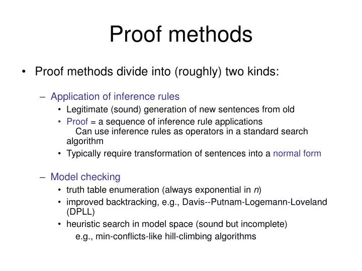
Proof methods. Proof methods divide into (roughly) two kinds: Application of inference rules Legitimate (sound) generation of new sentences from old Proof = a sequence of inference rule applications Can use inference rules as operators in a standard search algorithm

E N D
Proof methods • Proof methods divide into (roughly) two kinds: • Application of inference rules • Legitimate (sound) generation of new sentences from old • Proof = a sequence of inference rule applications Can use inference rules as operators in a standard search algorithm • Typically require transformation of sentences into a normal form • Model checking • truth table enumeration (always exponential in n) • improved backtracking, e.g., Davis--Putnam-Logemann-Loveland (DPLL) • heuristic search in model space (sound but incomplete) e.g., min-conflicts-like hill-climbing algorithms
Conversion to CNF B1,1 (P1,2 P2,1)β 1. Eliminate , replacing α β with (α β)(β α). (B1,1 (P1,2 P2,1)) ((P1,2 P2,1) B1,1) 2. Eliminate , replacing α β with α β. (B1,1 P1,2 P2,1) ((P1,2 P2,1) B1,1) 3. Move inwards using de Morgan's rules and double-negation: (B1,1 P1,2 P2,1) ((P1,2 P2,1) B1,1) 4. Apply distributivity law (V over ^) and flatten: (B1,1 P1,2 P2,1) (P1,2 B1,1) (P2,1 B1,1)
Resolution algorithm • Proof by contradiction, i.e., show KBα unsatisfiable
Resolution example • KB = (B1,1 (P1,2 P2,1)) B1,1 α = P1,2
Forward and backward chaining • Horn Form (restricted) KB = conjunction of Horn clauses • Horn clause = • proposition symbol; or • (conjunction of symbols) symbol • E.g., C (B A) (C D B) • Modus Ponens (for Horn Form): complete for Horn KBs α1, … ,αn, α1 … αnβ β • Can be used with forward chaining or backward chaining. • These algorithms are very natural and run in linear time
Forward chaining • Idea: fire any rule whose premises are satisfied in the KB, • add its conclusion to the KB, until query is found
Forward chaining algorithm • Forward chaining is sound and complete for Horn KB
Proof of completeness • FC derives every atomic sentence that is entailed by KB • FC reaches a fixed point where no new atomic sentences are derived • Consider the final state as a model m, assigning true/false to symbols • Every clause in the original KB is true in m a1 … ak b • Hence m is a model of KB • If KB╞ q, q is true in every model of KB, including m
Backward chaining Idea: work backwards from the query q: to prove q by BC, check if q is known already, or prove by BC all premises of some rule concluding q Avoid loops: check if new subgoal is already on the goal stack Avoid repeated work: check if new subgoal • has already been proved true, or • has already failed
Forward vs. backward chaining • FC is data-driven, automatic, unconscious processing, • e.g., object recognition, routine decisions • May do lots of work that is irrelevant to the goal • BC is goal-driven, appropriate for problem-solving, • e.g., Where are my keys? How do I get into a PhD program? • Complexity of BC can be much less than linear in size of KB
Efficient propositional inference Two families of efficient algorithms for propositional inference: Complete backtracking search algorithms • DPLL algorithm (Davis, Putnam, Logemann, Loveland) • Incomplete local search algorithms • WalkSAT algorithm
The DPLL algorithm Determine if an input propositional logic sentence (in CNF) is satisfiable. Improvements over truth table enumeration: • Early termination A clause is true if any literal is true. A sentence is false if any clause is false. • Pure symbol heuristic Pure symbol: always appears with the same "sign" in all clauses. e.g., In the three clauses (A B), (B C), (C A), A and B are pure, C is impure. Make a pure symbol literal true. • Unit clause heuristic Unit clause: only one literal in the clause The only literal in a unit clause must be true.
The WalkSAT algorithm • Incomplete, local search algorithm • Evaluation function: The min-conflict heuristic of minimizing the number of unsatisfied clauses • Balance between greediness and randomness
Hard satisfiability problems • Consider random 3-CNF sentences. e.g., (D B C) (B A C) (C B E) (E D B) (B E C) m = number of clauses n = number of symbols • Hard problems seem to cluster near m/n = 4.3 (critical point)
Hard satisfiability problems • Median runtime for 100 satisfiable random 3-CNF sentences, n = 50
Summary • Logical agents apply inference to a knowledge base to derive new information and make decisions • Basic concepts of logic: • syntax: formal structure of sentences • semantics: truth of sentences wrt models • entailment: necessary truth of one sentence given another • inference: deriving sentences from other sentences • soundness: derivations produce only entailed sentences • completeness: derivations can produce all entailed sentences • Resolution is complete for propositional logicForward, backward chaining are linear-time, complete for Horn clauses • Propositional logic lacks expressive power