Review of the Basic Logic of NHST

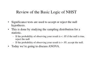
1. Review of the Basic Logic of NHST • Significance tests are used to accept or reject the null hypothesis. • This is done by studying the sampling distribution for a statistic. • If the probability of observing your result is < .05 if the null is true, reject the null • If the probability of observing your result is > .05, accept the null. • Today we’re going to discuss ANOVA.

2. ANOVA • A common situation in psychology is when an experimenter randomly assigns people to more than two groups to study the effect of the manipulation on a continuous outcome. • The significance test used in this kind of situation is called an ANOVA, which stands for analysis of variance.

3. ANOVA example • We are interested in whether peoples diet affects their happiness. • We take a sample of 60 people and randomly assign (a) 20 people to eat at least three fruits a day, (b) 20 people to eat at least three vegetables a day, and (c) 20 people to eat at least three donuts a day. • Subsequently we measure how happy people are on a continuous scale. • Note: The independent variable is categorical (people are assigned to groups); there are three groups total. • The dependent variable is continuous—we measure how happy people are on a continuous metric.

4. ANOVA example • Let’s say we find that the fruit group has a mean score of 3 ( =1), the veggie group has a mean score of 3.2 ( = .9), and the donut group has a mean score of 4.0 ( = 1.2). • Two possibilities • The differences between groups are due to sampling error, not a real effect of diet. In other words, the three samples are drawn from populations with identical means and variances. • The differences between groups are due to the effect of diet, not sampling error. In other words, the samples are drawn from populations with different means.

5. ANOVA example • In order to evaluate the null hypothesis, we need to know how likely it is that we would observe the differences we observed if the null hypothesis is true. • How can we do this? • As before, we construct a sampling distribution. • The sampling distribution used in ANOVA is conceptually different from the one used with a t-test.

6. F-ratio • The sampling distribution for a t-test was based on mean differences, and the t-distribution itself is based on mean differences relative to the sampling error. • In ANOVA, the sampling distribution is based on a ratio called the F-ratio. • The F-ratio is the ratio of the population variance as estimated between groups vs. within groups.

7. Variation in Sample Means drawn from the same population • We begin by noting that anytime we take random samples of the same size from a population, we will observe variation in our sample means—despite the fact that the samples come from the same population. • Why? This occurs because of sampling error. The sample is only a subset of the population, and, hence, only represents a portion of the scores composing the population.

8. Implications of the variation • What are the implications of sampling error in this context? • We will observe variability in the sample means for our fruit, veggie, and donut groups even if the null hypothesis is true. • How much variability will we observe? • This depends on two factors: • Sample size. As N increases, sampling error decreases. We’ll ignore this factor for now. • The variance of the scores in the population. When there is a lot of variation in happiness in the population, we’ll be more likely to observe variation among our sample means.

9. Estimating the variance in the population • Thus, our first step in conducting a significance test ANOVA-style is to estimate the variance of the dependent variable in the population. • PREVIEW: We’re going to use this information to determine whether the variation in sample means that we observe is greater than what we would expect if the samples all came from the same population. • We’re going to estimate this variance in two ways: within groups and between groups.

10. Method # 1 | Within Groups • How can we estimate the variance of the scores in the population? • We can draw on the logic of pooled variances that we discussed in the lecture on t-tests. • If the samples come from populations with identical means and variances, then each of the three sample variances is an estimate of the same quantity (i.e., the population variance). • Thus, we can pool or average the three variances (using the N-1 correction) to estimate the population variance.

11. MSWithin • In our example, we pool (i.e., average) 1, .9, and 1.2. • (1 + .9 + 1.2)/3 = 1.03 • Thus, our pooled estimate of the population variance is 1.03 • In ANOVA-talk, this pooled estimate of the population variance is called mean squares within or MSWithin. • We use the term “within” because we are estimating the population variance separately within each sample or condition.

12. Method # 2 | Between Groups • There is another way to estimate the variance in the population, based on studying the variation in sample means across or between conditions. • Recall from our discussion of sampling distributions of means that, given certain facts about the population and the sampling process, we could characterize the range of long-run sample outcomes. • For example, characterizes the average difference we might expect between sample means and the population mean.

13. Method # 2 • We can view our three sample (i.e., condition) means as constituting a “sampling distribution” of sorts based on three samples instead of an infinite number of samples (as is the case in a theoretical sampling distribution). • Hence, if we calculate the variance among these three sample means we’re essentially estimating the variance of the sampling distribution of means.

14. An approximate version of the theoretical sampling distribution based on the three means obtained in our study. The variance of these three means then provides an estimate of . Why is this cool? Because if we can estimate , then we have an estimate of (the population variance)!!! A theoretical sampling distribution of means based on infinite number of samples. This distribution has a standard deviation of or a variance of .

15. How do we do it? • Well, we have three sample means. To find the variance among them, we simply find the average squared difference among them. • First, we need to find the Grand Mean (GM): the mean of the three means • GM = (3 + 3.2 + 4)/3 = 3.4

16. How do we do it? • Now we can estimate the variance of the sampling distribution of means, and hence the variance of the population, by studying the average squared deviation of these three means from the Grand Mean. • Note: We use 1 less than the number of groups in the denominator for the same reason we use 1 less than the number of people when estimating a population variance: We are estimating a variance, albeit, the variance of a sampling distribution of means instead of a population variance. Any variance that is an estimate of a population variance will be a bit too small.

17. For our example M GM (M – GM) (M – GM)2 3 3.4 -.40 .16 3.2 3.4 -.20 .04 4 3.4 .60 .36 Ngroups = 3, so Ngroups –1 = 2 (M – GM)2 /2 = (.16 +.04+.36)/2 = .28

18. MSBetween • We’re almost there. • Now, we have an estimate of the variance of the sampling distribution, • We know that N (the sample size within a condition) is 20, so simple algebraic manipulation reveals that our estimate of the population variance is 5.6 • In short, we can estimate the population variance between samples by multiplying the variance among means by the sample size. • This quantity is called Mean Squares Between or MSBetween.

19. Getting to the big picture • Ok, we’ve been traveling some dark back roads. What does this all mean? • First, we should note that there are two ways to estimate the population variance from our three sample/condition means • MSWithin: We can pool the variance estimates that are calculated within each condition • MSBetween : We can treat the three sample means as if they comprise an approximate sampling distribution of means. By estimating the variance of this sampling distribution, we can also estimate the variance of the population.

20. F ratio • Now, here is the important part. • If the null hypothesis is true, then these two mathematically distinct estimates of the population variance should be identical. • If we express them as a ratio, the ratio should be close to 1.00.

21. F ratio • However—and this is critical—if the null hypothesis is false, and we are sampling from populations with different means, the variance between means will be greater than what we would observe if the null hypothesis was true. • The size of MSWithin, however, will be the same. (Footnote) • Thus, the F ratio will become increasingly larger than 1.00 as the difference between population means increases.

22. F ratio • Even if the null hypothesis is true, the F ratio will depart from 1 because of sampling error. • The degree to which it departs from 1, under various sample sizes, can be quantified probabilistically. • The significance test works as follows: When the p-value associated with the F-ratio for a specific sample size is < .05, we reject the null hypothesis. When it is larger than .05, we accept the null hypothesis.

23. F ratio our example • In our example, MSWithin was 1.03. MSBetween was 5.6. Thus, • If we were to look up some probability values in a table, we would find the p-value associated with this particular F is less than .05. Thus, we would reject the null hypothesis and conclude that diet has an effect on happiness.

24. Summary • ANOVA is a significance test the is frequently used when there are two or more conditions and a continuous outcome variable. • ANOVA is based on the comparison of two estimates of the population variance • When the null hypothesis is true, these two estimates will converge. • When the null hypothesis is false (i.e., the groups are being sampled from populations with different means), the two estimates will diverge, leading to an F ratio larger than 1. • When the p-value associated with an F-ratio calculated in a study is < .05, reject null. If not, accept null.