Download
1 / 70
710 likes | 866 Views
ROMS 4D-Var: Secrets Revealed. Andy Moore UC Santa Cruz. Ensemble 4D-Var. f b , B f. ROMS. Obs y, R. h , Q. b b , B b. x b , B. 4D-Var. dof. Adjoint 4D-Var. impact. Priors & Hypotheses. Hypothesis Tests. Posterior. Uncertainty. Analysis error. Forecast. Term balance,

E N D
ROMS 4D-Var: Secrets Revealed Andy Moore UC Santa Cruz
Ensemble 4D-Var fb, Bf ROMS Obs y, R h, Q bb, Bb xb, B 4D-Var dof Adjoint 4D-Var impact Priors & Hypotheses Hypothesis Tests Posterior Uncertainty Analysis error Forecast Term balance, eigenmodes Clipped Analyses Ensemble (SV, SO) ROMS 4D-Var
ROMS 4D-Var • Incremental (linearize about a prior) (Courtier et al, 1994) • Primal & dual formulations (Courtier 1997) • Primal – Incremental 4-Var (I4D-Var) • Dual – PSAS (4D-PSAS) & indirect representer (R4D-Var) (Da Silva et al, 1995; Egbert et al, 1994) • Strong and weak (dual only) constraint • Preconditioned, Lanczos formulation of conjugate gradient (Lorenc, 2003; Tshimanga et al, 2008; Fisher, 1997) • Diffusion operator model for prior covariances (Derber & Bouttier, 1999; Weaver & Courtier, 2001) • Multivariate balance for prior covariance (Weaver et al, 2005) • Physical and ecosystem components • Parallel (MPI)
The Secrets… • The adjoint operator • Matrix-less iterations • Lanczos algorithm
Can you solve these equations? There are infinite possibilities!
Look for solutions of the form: Generating vector …there is a Natural Solution
Identifies the part of 3-space that is activated by y Two Spaces A is a 2×3 matrix y and s reside in “2-space” x resides in “3-space” A maps from 3-space to 2-space ATis a 3×2 matrix ATmaps from 2-space to 3-space
Think of x as corrections to the prior/background This looks lot like the ocean state estimation problem… Ocean state Ocean Observations Insufficient observations to uniquely determine elements of x Use ATto identify the natural solution
Notation Ocean state vector:
Prior (background) circulation estimate: Observations: Posterior (analysis) circulation estimate: Observation matrix Data Assimilation: Recap Gain Matrix
Posterior (analysis) circulation estimate: Innovation vector: Data Assimilation: Recap Adjoint plays a key role in identifying K
Posterior, xa Data Assimilation: Recap fb(t), Bf Prior bb(t), Bb xb(0), B Obs, y Prior, xb x(t) time Model solutions depends on xb(0), fb(t), bb(t), h(t)
More Notation & Nomenclature Prior Innovation vector State vector Control vector Observation vector h(t) = Correction for model error h(t)=0 : Strong constraint h(t)≠0 : Weak constraint Observation matrix
Conditional Probability: Background error covariance Variational Data Assimilation: Recap Observation error covariance J is called the “cost” or “penalty” function. Problem: Find z=za that minimizes J (i.e. maximizes P) za is the “maximum likelihood” or “minimum variance” estimate.
initial condition increment corrections for model error boundary condition increment forcing increment Incremental Formulation fb(t), Bf Prior bb(t), Bb xb(0), B Tangent Linear Model sampled at obs points Obs Error Cov. Innovation Background error covariance
Two Spaces G samples the tangent linear model at observation points. G maps from model (primal) space to observation (dual) space GTmaps from observation (dual) space to model (primal) space
initial condition increment corrections for model error boundary condition increment forcing increment Variational Data Assimilation fb(t), Bf Prior bb(t), Bb xb(0), B Find dz that minimizes J: using principles of variational calculus (“Var”)
The Solution! Analysis: Gain (dual): Gain (primal):
Two Spaces Gain (dual): Gain (primal):
Two Spaces G maps from model (primal) space to observation (dual) space GTmaps from observation (dual) space to model (primal) space
Recall the Solutions Analysis: Gain (dual): Gain (primal):
Equivalent Linear Systems Dual: Primal:
Iterative Solution of Linear Equations General form: Find s that minimizes: At the minimum:
Conjugate Gradient (CG) Methods Contours of J
Looks, feels & smells like matrix… Dual: Primal:
Matrix-less Operations There are no matrix multiplications! Zonal shear flow
Matrix-less Operations There are no matrix multiplications! Adjoint Model Zonal shear flow
Matrix-less Operations There are no matrix multiplications! Adjoint Model Zonal shear flow
Matrix-less Operations There are no matrix multiplications! Adjoint Model Zonal shear flow
Matrix-less Operations There are no matrix multiplications! Covariance Zonal shear flow
Matrix-less Operations There are no matrix multiplications! Covariance Zonal shear flow
Matrix-less Operations There are no matrix multiplications! Tangent Linear Model Zonal shear flow
Matrix-less Operations There are no matrix multiplications! Tangent Linear Model Zonal shear flow
Matrix-less Operations = A representer Green’s Function A covariance Zonal shear flow
Matrix-less Operations There are no matrix multiplications! Tangent Linear Model Zonal shear flow
fb(t), Bf bb(t), Bb xb(0), B Previous assimilation cycle The Priors for ROMS CCS COAMPS forcing ECCO open boundary conditions 30km, 10 km & 3 km grids, 30- 42 levels Veneziani et al (2009) Broquet et al (2009)
Observations (y) CalCOFI & GLOBEC SST & SSH Ingleby and Huddleston (2007) TOPP Elephant Seals Argo Data from Dan Costa
4D-Var Performance Primal, strong 3-10 March, 2003 (10km, 42 levels) Dual, strong Dual, weak Jmin
The Beauty of Lanczos Cornelius Lanczos (1893-1974)
Conjugate Gradient (CG) Methods Contours of J
Recall the Solutions Analysis: Gain (dual): Gain (primal): Dual Lanczos vectors Primal Lanczos vectors
Endless Possibilties? • Posterior error • Posterior EOFs • Preconditioning • Degrees of freedom • Array modes • Observation impact • Observation sensitivity • Think outside the box…
Ensemble 4D-Var fb, Bf ROMS Obs y, R h, Q bb, Bb xb, B 4D-Var dof Adjoint 4D-Var impact Priors & Hypotheses Hypothesis Tests Posterior Uncertainty Analysis error Forecast Term balance, eigenmodes Clipped Analyses Ensemble (SV, SO) ROMS 4D-Var