Download
1 / 21
210 likes | 327 Views
Calculations for Decision Tree. Today we present the “folding back” procedure for analyzing decision trees Two main ideas Look Forward : Early observations change prior estimates of events => changes in decisions you might have made without information

E N D
Calculations for Decision Tree • Today we present the “folding back” procedure for analyzing decision trees • Two main ideas • Look Forward: Early observations change prior estimates of events => changes in decisions you might have made without information • Look Back: Analysis from last stages going toward front => “folding back”
Components of Decision Tree • Structure • Sequence of Choices; Possible outcomes • Data • Uncertainties; Value of Each Possible Outcome • Analysis Results • Revision of Probabilities based on observations • Expected Values at Each Stage • Best Choices at Each Stage • Best Choice for all Stages Decision Tree Structure
Review of 1- stage layout EV (raincoat) = 0.8 = 2.0 - 1.2 EV (no raincoat) = - 1.6 = - 4.0 + 2.4
Sequence of Alternatives – 2 stages • We repeat basic block (changing entries) Notice: Data seen in early stages => changes later probabilities, results
Looking Forward • Look Forward: Early observations change prior estimates of events • We observe information as time moves on • Either passively: see the price of oil change • Actively: We create situations to look for new data • For Example? • Turn on weather report • Distribute beta version • Run prototype plant • These data => Revision of later probabilities
Calculations for Looking Forward • At start we have estimates of future states • These are the “prior” probabilities • When we see what happens, • These are the “Observations” O for Bayes Theorem • To the extent that we have conditional probability between Observations and State of interest and Probability of Observation [These are the P(O/E) and the P(O)] • We can revise the Probabilities for future stages
Forward Calculations = Big Job • This discussion will be taken up next session • Updating probabilities based on observations is a central part of valuing flexibility in design • For clarity of presentation, we defer the “looking forward” calculations until after we understand basic analysis of decision trees • For now we will look at an example where these calculations for the revision of probabilities does not come into play
Looking Backward • This is the standard approach to analyzing decision trees • But it is “counter-intuitive” • The object of a decision analysis is to determine the best policy of choice or action: what should we do first, second, third… • This is forward-looking… going into future • BUT: analysis starts in future and works back!
Background to Concept • Consider a situation that in each stage has: • 2 decisions to be made, • each with 3 outcomes • thus with 6 possible combinations (or paths) • The number of combinations squares at each stage • The total number of possibilities, looking ahead from the start, is thus 6N • It is time-consuming, and confusing, to think about all these combinations, even for a simple problem
Looking Back Concept • Instead of looking forward at all possible combinations over N stages… • Which is a big, massive problem • We get solution by repeating a simple process many times • Advantage 1: Calculation easy • Advantage 2: Size of Problem is linear in number stages [ f(N) ] rather than exponential [ f(x)N ]
Looking Back Process • Instead of looking forward at all possible combinations over N stages… • We start analysis at last, Nth, stage where • Few combinations for each possible result from (N-1)th stage (e.g., 2 choices and 6 outcomes) • So choice easy, • Even though process repeated for each (N-1)th outcome • We then know best choices for (N -1)th stage • We repeat this process until we get to beginning • We get solution by repeating a simple process
Preview of Dynamic Programming • The looking back process for decision trees is … particular case of a larger class of techniques • “Dynamic Programming” is name of this larger class • Dynamic Programming approach in general will be presented later • DP is also the basis for “lattice analysis”, one of two main ways to analyze flexibility in design
A Simple Example • Inspired by Katherine Dykes http://ardent.mit.edu/real_options/Real_Options_Papers/Dykes_Wind_Farm_08.pdf • Region has 3 initial choices for a wind farm • Big – cheaper when fully utilized due to E of Scale • Small – without Economies of Scale • At end of 1st stage, they will know if Carbon Tax law passed – which would increase value of farm • In 2nd stage, they could expand farm to big size
Decision Tree for example Outcome values assumed Data in tree to be filled in as example develops
Nth (second) Stage for Example • The analysis for the second stage in the example has been simplified to avoid tedious repetition • Specifically, there are no chance events in this version of the case. It is assumed – contrary to any real situation – that the value of any plant is known once the possibility of the “Carbon Tax” has been resolved. • Thus the best decision in second stage is obvious • The value of the best decision is entered as the outcome for the previous stage (in bigger font)
Results after Analysis of Last Stage The best choices in the last stage (the second in this case) highlighted and entered as outcomes for previous stage (the first, here)
Results for Stage with Chance Events • This example assumes that chance event and its probability are independent decisions made • Such an assumption reasonable in many cases, here because decision to build wind farm unlikely to change probability of new law • However, contrary often true (example: volume of sales affected by advertising decisions) • In this case, assumed probability of carbon tax favorable to wind far was 0.4
Results for First Stage Value of any decision is the expectation of its outcomes. Value (Big) = .4(25) + .6(-5) = 7 Note: best value (= 10.8) is an expectation over actual results (here 18 and 6)
Results of Analysis • An optimal Expected Value • Here: 10.8 -- but this is not a result that will be seen • An Optimal first choice • Here: Build Medium Size Facility • A Strategy: • First, build Medium, then • If Carbon Tax passes, Expand (Build Big0 • If Tax not passed, Stay at Medium Size • Second-best solution • If we knew Tax would pass, Best choice is Build Big from start
Why is process called “folding back”? Starting at the “back” the analysis eliminates, “folds” , dominated decisions, simplifying the tree
Summary • Decision trees best analyzed by process of “folding back” • This process is efficient because it • Simplifies the analysis • Much more efficient: Size linear – not exponential – in number of stages • This process illustrates a fundamental way in which we can analyze combinations of sequences of choices. • Dynamic Programming generalizes the approach