Download
1 / 32

E N D
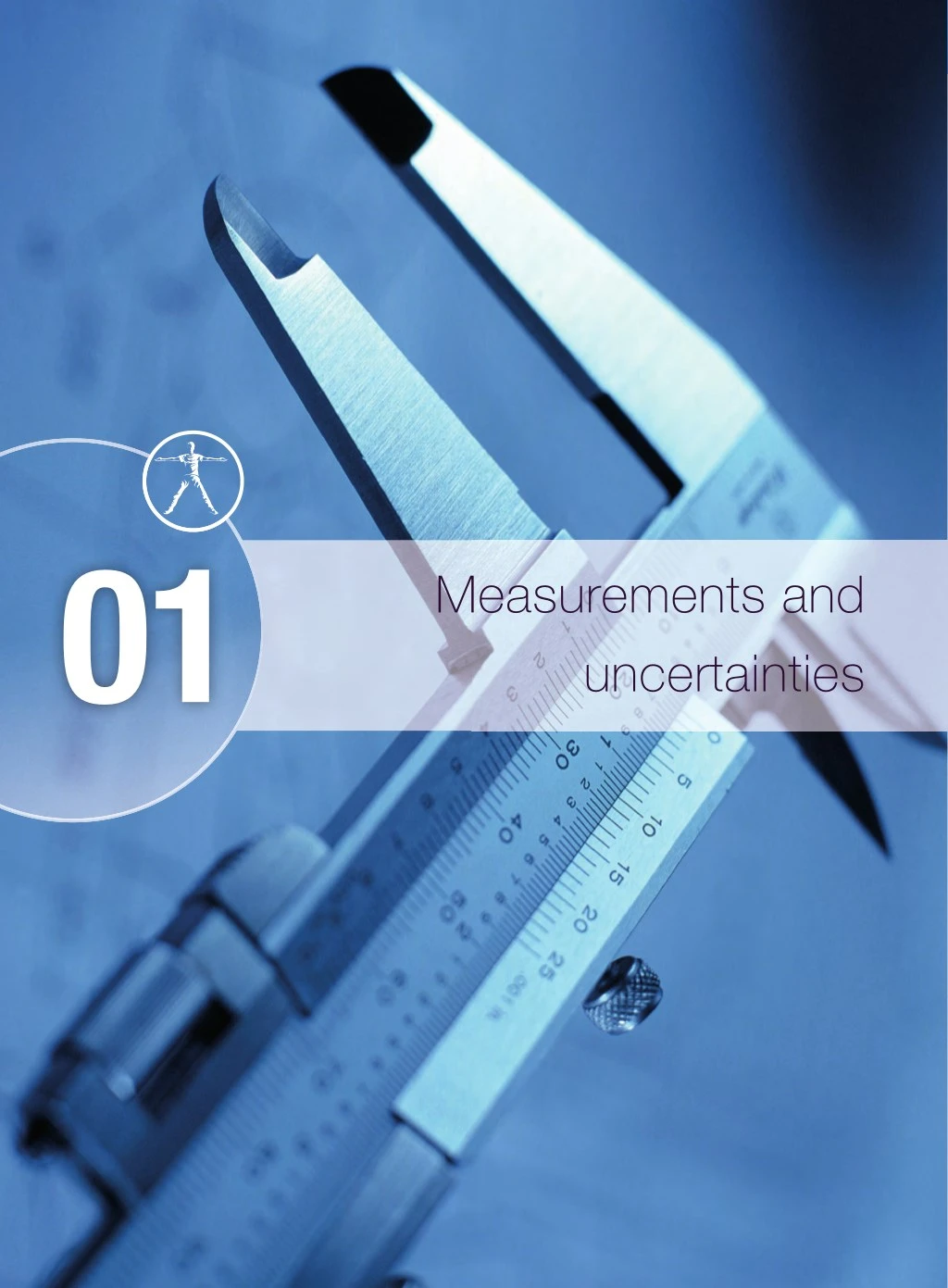
01 Measurements and uncertainties M01_IBPH_SB_IBGLB_9021_CH01.indd 2 25/03/2014 13:47
Essential ideas 1.1 Since 1948, the Système International d’Unités (SI) has been used as the preferred language of science and technology across the globe and refl ects current best measurement practice. A common standard approach is necessary so units ‘are readily available to all, are constant through time and space, and are easy to realize with high accuracy’ – France: Bureau International des Poids et Mesures, organisation intergouvernementale de la Convention du Mètre, The International System of Units (SI), Bureau International des Poids et Mesures, March 2006. Web: 21 May 2012. If used properly a Vernier calliper can measure small lengths to within ±0.02 mm. Measurements in physics Since 1948, the Système International d’Unités (SI) has been used globe and refl ects current best measurement practice. A common standard approach is necessary so units ‘are readily available to all, are constant through time and space, and are easy to realize with high accuracy’ – France: Bureau International des Poids et Mesures, The Bureau International des Poids et 1.2 Uncertainties and errors Scientists aim towards designing experiments that can give a ‘true value’ from their measurements, but due to the limited precision in measuring devices they often quote their results with some form of uncertainty. Scientists aim towards designing experiments that can give a ‘true value’ from their measurements, but due to the limited precision in measuring 1.3 Vectors and scalars Some quantities have direction and magnitude, others have magnitude only, and this understanding is key to correct manipulation of quantities. This subtopic will have broad applications across multiple fi elds within physics and other sciences. manipulation of quantities. This subtopic will have broad applications NATURE OF SCIENCE Physics is about modelling the physical Universe so that we can predict outcomes but before we can develop models we need to defi ne quantities and measure them. To measure a quantity we fi rst need to invent a measuring device and defi ne a unit. When measuring we should try to be as accurate as possible but we can never be exact, measurements will always have uncertainties. This could be due to the instrument or the way we use it or it might be that the quantity we are trying to measure is changing. 1.1 Measurements in physics 1.1 Measurements in physics Understandings, applications, and skills: Fundamental and derived SI units ●Using SI units in the correct format for all required measurements, fi nal answers to calculations and presentation of raw and processed data. Guidance ●SI unit usage and information can be found at the website of Bureau International des Poids et Mesures. Students will not need to know the defi nition of SI units except where explicitly stated in the relevant topics. Candela is not a required SI unit for this course. Scientifi c notation and metric multipliers ●Using scientifi c notation and metric multipliers. Signifi cant fi gures Orders of magnitude ●Quoting and comparing ratios, values, and approximations to the nearest order of magnitude. Estimation ●Estimating quantities to an appropriate number of signifi cant fi gures. Mesures. Students will not need to know the defi nition of SI units except where explicitly stated in the 3 M01_IBPH_SB_IBGLB_9021_CH01.indd 3 25/03/2014 13:47
01 Measurements and uncertainties Making observations Before we can try to understand the Universe we have to observe it. Imagine you are a cave man/woman looking up into the sky at night. You would see lots of bright points scattered about (assuming it is not cloudy). The points are not the same but how can you describe the differences between them? One of the main differences is that you have to move your head to see different examples. This might lead you to def ne their position. Occasionally you might notice a star f ashing so would realize that there are also differences not associated with position, leading to the concept of time. If you shift your attention to the world around you you’ll be able to make further close-range observations. Picking up rocks you notice some are easy to pick up while others are more diff cult; some are hot, some are cold, and different rocks are different colours. These observations are just the start: to be able to understand how these quantities are related you need to measure them but before you do that you need to be able to count. Figure 1.1 Making observations came before science. Numbers Numbers weren’t originally designed for use by physics students: they were for counting objects. If the system of numbers had been totally different, would our models of the Universe be the same? 2 apples + 3 apples = 5 apples 2 + 3 = 5 2 × 3 apples = 6 apples 6 apples 2 = 3 apples So the numbers mirror what is happening to the apples. However, you have to be careful: you can do some operations with numbers that are not possible with apples. For example: (2 apples)2 = 4 square apples? 4 M01_IBPH_SB_IBGLB_9021_CH01.indd 4 25/03/2014 13:47
Standard form In this course we will use some numbers that are very big and some that are very small. 602 000 000 000 000 000 000 000 is a commonly used number as is 0.000 000 000 000 000 000 16. To make life easier we write these in standard form. This means that we write the number with only one digit to the left of the decimal place and represent the number of zeros with powers of 10. It is also acceptable to use a prefi x to denote powers of 10. Prefi x Value 1012 T (tera) 109 G (giga) So 106 M (mega) 103 k (kilo) 602 000 000 000 000 000 000 000 = 6.02 × 10²³ (decimal place must be shifted right 23 places) 10–2 c (centi) 10–3 m (milli) 0.000 000 000 000 000 000 16 = 1.6 × 10⁻¹⁹ (decimal place must be shifted left 19 places). 10–6 µ (micro) Exercise 10–9 n (nano) 1 Write the following in standard form. (a) 48 000 (b) 0.000 036 (c) 14 500 (d) 0.000 000 48 10–12 p (pico) 10–15 f (femto) If you set up your calculator properly it will always give your answers in standard form. Measurement We have seen that there are certain fundamental quantities that def ne our Universe. These are position, time, and mass. Distance Before we take any measurements we need to def ne the quantity. The quantity that we use to def ne the position of different objects is distance. To measure distance we need to make a scale and to do that we need two f xed points. We could take one f xed point to be ourselves but then everyone would have a different value for the distance to each point so we take our f xed points to be two points that never change position, for example the ends of a stick. If everyone then uses the same stick we will all end up with the same measurement. We can’t all use the same stick so we make copies of the stick and assume that they are all the same. The problem is that sticks aren’t all the same length, so our unit of length is now based on one of the few things we know to be the same for everyone: the speed of light in a vacuum. Once we have def ned the unit, in this case the metre, it is important that we all use it (or at least make it very clear if we are using a different one). There is more than one system of units but the one used in this course is the SI system (International system). Here are some examples of distances measured in metres. The distance from Earth to the Sun = 1.5 × 10¹¹ m The size of a grain of sand = 2 × 10⁻⁴ m The distance to the nearest star = 4 × 10¹⁶ m The radius of the Earth = 6.378 × 10⁶ m Realization that the speed of light in a vacuum is the same no matter who measures it led to the speed of light being the basis of our unit of length. The metre The metre was originally defi ned in terms of several pieces of metal positioned around Paris. This wasn’t very accurate so now one metre is defi ned as the distance travelled by light in a vacuum in 299 792 458 of a second. 1 Exercise 2 Convert the following into metres (m) and write in standard form: (a) Distance from London to New York = 5585 km. (b) Height of Einstein was 175 cm. (c) Thickness of a human hair = 25.4 μm. (d) Distance to furthest part of the observable Universe = 100 000 million million million km. 5 M01_IBPH_SB_IBGLB_9021_CH01.indd 5 25/03/2014 13:47
01 Measurements and uncertainties Time When something happens we call it an event. To distinguish between different events we use time. The time between two events is measured by comparing to some f xed value, the second. Time is also a fundamental quantity. The second The second was originally defi ned as a fraction of a day but today’s defi nition is ‘the duration of 9 192 631 770 periods of the radiation corresponding to the transition between the two hyperfi ne levels of the ground state of the caesium-133 atom’. Some examples of times: Time for the Moon to go around the Earth = 1 month Time between beats of a human heart = 1 s Time for the Earth to go around the Sun = 1 year Exercise 3 Convert the following times into seconds (s) and write in standard form: (a) 85 years, how long Newton lived. (b) 2.5 ms, the time taken for a mosquito’s wing to go up and down. (c) 4 days, the time it took to travel to the Moon. (d) 2 hours 52 min 59 s, the time for Concord to fly from London to New York. If nothing ever happened, would there be time? Mass If we pick different things up we f nd another difference. Some things are easy to lift up and others are diff cult. This seems to be related to how much matter the objects consist of. To quantify this we def ne mass measured by comparing different objects to a piece of metal in Paris, the standard kilogram. The kilogram The kilogram is the only fundamental quantity that is still based on an object kept in Paris. Moves are underway to change the defi nition to something that is more constant and better defi ned but does it really matter? Would anything change if the size of the ‘Paris mass’ changed? Some examples of mass: Approximate mass of a man = 75 kg Mass of the Earth = 5.97 × 1024 kg Mass of the Sun = 1.98 × 1030 kg Exercise 4 Convert the following masses to kilograms (kg) and write in standard form: (a) The mass of an apple = 200 g. (b) The mass of a grain of sand = 0.00001 g. (c) The mass of a family car = 2 tonnes. Volume The space taken up by an object is def ned by the volume. Volume is measured in cubic metres (m3). Volume is not a fundamental unit since it can be split into smaller units (m × m × m). We call units like this derived units. Exercises 5 6 Calculate the volume of a room of length 5 m, width 10 m, and height 3 m. Using the information from page 5, calculate: (a) the volume of a human hair of length 20 cm. (b) the volume of the Earth. Density By measuring the mass and volume of many different objects we f nd that if the objects are made of the same material, the ratio mass/volume is the same. This quantity is called the density. The unit of density is kg m–3. This is another derived unit. 6 M01_IBPH_SB_IBGLB_9021_CH01.indd 6 25/03/2014 13:47
Examples include: Density of water = 1.0 × 10³ kg m–3 Density of air = 1.2 kg m–3 Density of gold = 1.93 × 10⁴ kg m–3 Exercises 7 8 9 Calculate the mass of air in a room of length 5 m, width 10 m, and height 3 m. Calculate the mass of a gold bar of length 30 cm, width 15 cm, and height 10 cm. Calculate the average density of the Earth. Displacement So far all that we have modelled is the position of objects and when events take place, but what if something moves from one place to another? To describe the movement of a body, we def ne the quantity displacement. This is the distance moved in a particular direction. N C A B The unit of displacement is the same as length: the metre. Example: Refering to the map in Figure 1.2: If you move from B to C, your displacement will be 5 km north. If you move from A to B, your displacement will be 4 km west. 5km Figure 1.2 Displacements on a map. Angle When two straight lines join, an angle is formed. The size of the angle can be increased by rotating one of the lines about the point where they join (the vertex) as shown in Figure 1.3. To measure angles we often use degrees. Taking the full circle to be 360° is very convenient because 360 has many whole number factors so it can be divided easily by e.g. 4, 6, and 8. However, it is an arbitrary unit not related to the circle itself. Figure 1.3 The angle between two lines. A s r θ B If the angle is increased by rotating line A the arc lengths will also increase. So for this circle we could use the arc length as a measure of angle. The problem is that if we take a bigger circle then the arc length for the same angle will be greater. We therefore def ne the angle by using the ratio s r which will be the same for all circles. This unit is the radian. For one complete circle the arc length is the circumference = 2πr so the angle 360° in radians = 2πr r = 2π. So 360° is equivalent to 2π. Since the radian is a ratio of two lengths it has no units. Summary of SI units The International System of units is the set of units that are internationally agreed to be used in science. It is still OK to use other systems in everyday life (miles, pounds, Fahrenheit) but in science we must always use SI. There are seven fundamental (or base) quantities. 7 M01_IBPH_SB_IBGLB_9021_CH01.indd 7 25/03/2014 13:47
01 Measurements and uncertainties Table 1.1 The seven fundamental quantities and their units. Base quantity Unit Symbol length metre m mass kilogram kg time second s electric current ampere A thermodynamic temperature kelvin K amount of substance mole mol luminous intensity candela cd The candela will not be used in this course. All other SI units are derived units; these are based on the fundamental units and will be introduced and def ned where relevant. So far we have come across just two. Table 1.2 Some SI derived quantities. Derived quantity Symbol Base units m3 volume m × m × m kg m × m × m kg m–3 density 1.2 Uncertainties and errors 1.2 Uncertainties and errors Understandings, applications, and skills: Random and systematic errors ●Explaining how random and systematic errors can be identifi ed and reduced. Absolute, fractional, and percentage uncertainty ●Collecting data that include absolute and/or fractional uncertainties and stating these as an uncertainty range (expressed as: [best estimate] ± [uncertainty range]). Guidance ●Analysis of uncertainties will not be expected for trigonometric or logarithmic functions in examinations. Error bars ●Propagating uncertainties through calculations involving addition, subtraction, multiplication, division, and raising to a power. Uncertainty of gradient and intercepts ●Determining the uncertainty in gradients and intercepts. NATURE OF SCIENCE In physics experiments we always quote the uncertainties in our measurements. Shops also have to work within given uncertainties and will be prosecuted if they overestimate the weight of something. When counting apples we can say there are exactly 6 apples but if we measure the length of a piece of paper we cannot say that it is exactly 21 cm wide. All measurements have an associated uncertainty and it is important that this is also quoted with the value. Uncertainties can’t be avoided but by carefully using accurate instruments they can be minimized. Physics is all about relationships between different quantities. If the uncertainties in measurement are too big then relationships are diffi cult to identify. Throughout the practical part of this course you will be trying to fi nd out what causes the uncertainties in your measurements. Sometimes you will be able to reduce them and at other times not. It is quite alright to have big uncertainties but completely unacceptable to manipulate data so that it appears to fi t a predicted relationship. 8 M01_IBPH_SB_IBGLB_9021_CH01.indd 8 25/03/2014 13:47
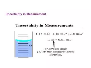
Uncertainty and error in measurement The SI system of units is def ned so that we all use the same sized units when building our models of the physical world. However, before we can understand the relationship between different quantities, we must measure how big they are. To make measurements we use a variety of instruments. To measure length, we can use a ruler and to measure time, a clock. If our f ndings are to be trusted, then our measurements must be accurate, and the accuracy of our measurement depends on the instrument used and how we use it. Consider the following examples. Even this huge device at CERN has uncertainties. Estimating uncertainty When using a scale such as a ruler the uncertainty in the reading is half of the smallest division. In this case the smallest division is 1 mm so the uncertainty is 0.5 mm. When using a digital device such as a balance we take the uncertainty as the smallest digit. So if the measurement is 20.5 g the uncertainty is ±0.1 g. Measuring length using a ruler Example 1 A good straight ruler marked in mm is used to measure the length of a rectangular piece of paper as in Figure 1.4. cm 0 1 2 3 4 5 6 7 The ruler measures to within 0.5 mm (we call this the uncertainty in the measurement) so the length in cm is quoted to 2 dp. This measurement is precise and accurate. This can be written as 6.40 ± 0.05 cm which tells us that the actual value is somewhere between 6.35 and 6.45 cm. Figure 1.4 Length = 6.40 ± 0.05 cm. If you measure the same thing many times and get the same value, then the measurement is precise. If the measured value is close to the expected value, then the measurement is accurate. If a football player hit the post 10 times in a row when trying to score a goal, you could say the shots are precise but not accurate. Example 2 Figure 1.5 shows how a ruler with a broken end is used to measure the length of the same piece of paper. When using the ruler, you fail to notice the end is broken and think that the 0.5 cm mark is the zero mark. This measurement is precise since the uncertainty is small but is not accurate since the value 6.90 cm is wrong. 1 2 3 4 5 6 7 Figure 1.5 Length = / 6.90 ± 0.05 cm. 9 M01_IBPH_SB_IBGLB_9021_CH01.indd 9 25/03/2014 13:47
01 Measurements and uncertainties Example 3 A cheap ruler marked only in 1 used to measure the length of the paper as in Figure 1.6. 2 cm is cm 0 1 2 3 4 5 6 7 These measurements are not precise but accurate, since you would get the same value every time. 7 Figure 1.6 6 Length = 6.5 ± 0.25 cm. 5 Example 4 In Figure 1.7, a good ruler is used to measure the maximum height of a bouncing ball. Even though the ruler is good it is very diff cult to measure the height of the bouncing ball. Even though you can use the scale to within 0.5 mm, the results are not precise (may be about 4.2 cm). However, if you do enough runs of the same experiment, your f nal answer could be accurate. 4 3 2 1 cm Precision and accuracy To help understand the difference between precision and accuracy, consider the four attempts to hit the centre of a target with 3 arrows shown in Figure 1.8. Figure 1.7 Height = 4.2 ± 0.2 cm A B C D Figure 1.8 Precise or Precise and accurate Precise but not accurate Not precise but accurate Not precise and not accurate accurate? A The arrows were f red accurately at the centre with great precision. B The arrows were f red with great precision as they all landed near one another, but not very accurately since they are not near the centre. C The arrows were not f red very precisely since they were not close to each other. However, they were accurate since they are evenly spread around the centre. The average of these would be quite good. D The arrows were not f red accurately and the aim was not precise since they are far from the centre and not evenly spread. So precision is how close to each other a set of measurements are and the accuracy is how close they are to the actual value. Errors in measurement There are two types of measurement error – random and systematic. It is not possible to measure anything exactly. This is not because our instruments are not exact enough but because the quantities themselves do not exist as exact quantities. Random error If you measure a quantity many times and get lots of slightly different readings then this called a random error. For example, when measuring the bounce of a ball it is very diff cult to get the same value every time even if the ball is doing the same thing. 10 M01_IBPH_SB_IBGLB_9021_CH01.indd 10 25/03/2014 13:47
Systematic error This is when there is something wrong with the measuring device or method. Using a ruler with a broken end can lead to a ‘zero error’ as in Example 2 on page 9. Even with no random error in the results, you’d still get the wrong answer. Reducing errors To reduce random errors you can repeat your measurements. If the uncertainty is truly random, they will lie either side of the true reading and the mean of these values will be close to the actual value. To reduce a systematic error you need to f nd out what is causing it and correct your measurements accordingly. A systematic error is not easy to spot by looking at the measurements, but is sometimes apparent when you look at the graph of your results or the f nal calculated value. Adding uncertainties If two values are added together then the uncertainties also add. For example, if we measure two lengths L1 = 5.0 ± 0.1 cm and L2 = 6.5 ± 0.1 cm then the maximum value of L1 is 5.1 cm and the maximum value of L2 is 6.6 cm so the maximum value of L1 + L2 = 11.7 cm. Similarly, the minimum value is 11.3 cm. We can therefore say that L1 + L2 = 11.5 ± 0.2 cm. then Δy = Δa + Δb y = a ± b If If you multiply a value by a constant then the uncertainty is also multiplied by the same number. 1 2L1 = 2.50 ± 0.05 cm. 2L1 = 10.0 ± 0.2 cm and So Example of measurement and uncertainties Let us consider an experiment to measure the mass and volume of a piece of plasticine (modelling clay). To measure mass we can use a top pan balance so we take a lump of plasticine and weigh it. The result is 24.8 g. We can repeat this measurement many times and get the same answer; there is no variation in the mass so the uncertainty in this measurement is the same as the uncertainty in the scale. The smallest division on the balance used is 0.1 g so the uncertainty is ±0.1 g. So mass = 24.8 ±0.1 g. To measure the volume of the plasticine we f rst need to mould it into a uniform shape: let’s roll it into a sphere. To measure the volume of the sphere we measure its diameter (V = 4πr3 3). Making an exact sphere out of the plasticine isn’t easy; if we do it many times we will get different shaped balls with different diameters so let’s try rolling the ball 5 times and measuring the diameter each time with a ruler. Ball of plasticine measured with a ruler. Using the ruler, we can only judge the diameter to the nearest mm so we can say that the diameter is 3.5 ± 0.1 cm. It is actually even worse than this since we also have to line up the zero at the other end, so 3.5 ± 0.2 cm might be a more reasonable estimate. If we turn the ball round we get the same value for d. If we squash the ball and make a new one we will still get a value of 3.5 ± 0.2 cm. This is not because the ball is perfect sphere every time but because our method of measurement isn’t sensitive enough to measure the difference. 11 M01_IBPH_SB_IBGLB_9021_CH01.indd 11 25/03/2014 13:47
01 Measurements and uncertainties Let us now try measuring the ball with a vernier calliper. A vernier calliper has sliding jaws which are moved so they touch both sides of the ball. The vernier calliper can measure to the nearest 0.002 cm. Repeating measurements of the diameter of the same lump of plasticine might give the results in Table 1.3. Table 1.3 Measurements of the diameter of a lump of Diameter/cm 3.640 3.450 3.472 3.500 3.520 3.520 3.530 3.530 3.432 plasticine. 3.540 3.550 3.550 3.560 3.560 3.570 3.572 3.582 3.582 The reason these are not all the same is because the ball is not perfectly uniform and if made several times will not be exactly the same. We can see that there is a spread of data from 3.400 cm to 3.570 cm with most lying around the middle. This can be shown on a graph but f rst we need to group the values as in Table 1.4. Distribution of measurements Figure 1.9 Distribution of measurements of diameter. 9 number of measurements 8 7 6 Range/cm No. of values within range 5 4 3.400–3.449 1 3 3.450–3.499 2 2 3.500–3.549 6 3.550–3.599 8 1 3.600–3.649 1 0 3.35 3.40 3.45 3.50 3.55 3.60 Table 1.4. diameter/cm 12 M01_IBPH_SB_IBGLB_9021_CH01.indd 12 25/03/2014 13:47
Even with this small sample of measurements you can see in Figure 1.9 that there is a spread of data: some measurements are too big and some too small but most are in the middle. With a much larger sample the shape would be closer to a ‘normal distribution’ as in Figure 1.10. Figure 1.10 Normal distribution curve. 900 number of measurements 800 700 600 500 400 300 200 100 0 3.35 3.40 3.45 3.50 3.55 3.60 3.65 diameter/cm The mean At this stage you may be wondering what the point is of trying to measure something that doesn’t have a def nite value. Well, we are trying to f nd the volume of the plasticine using the formula V = 4πr3 3. This is the formula for the volume of a perfect sphere. The problem is we can’t make a perfect sphere; it is probably more like the shape of an egg so depending on which way we measure it, sometimes the diameter will be too big and sometimes too small. Now it is just as likely to be too big as too small so if we take the mean of all our measurements we should be close to the ‘perfect sphere’ value which will give us the correct volume of the plasticine. The mean or average is found by adding all the values and dividing by the number of values. In this case the mean = 3.537 cm. This is the same as the peak in the distribution. We can check this by measuring the volume in another way; for example, sinking it in water and measuring the volume displaced. Using this method gives a volume = 23 cm3. Rearranging the formula gives r = 3 3V 4π. Substituting for V gives d = 3.53 cm which is fairly close to the mean. Calculating the mean reduces the random error in our measurement. There is a very nice example of this that you might like to try with your friends. Fill a jar with jellybeans and get your friends to guess how many there are. Assuming that they really try to make an estimate rather than randomly saying a number, the guesses are just as likely to be too high as too low. So, if after you collect all the data you f nd the average value, it should be quite close to the actual number of beans. 13 M01_IBPH_SB_IBGLB_9021_CH01.indd 13 25/03/2014 13:47
01 Measurements and uncertainties Standard deviation The standard deviation tells us how spread out the data is from the mean. It is calculated by using the following formula: Δx/cm Δx2/cm2 x/cm 3.432 −0.105 0.010 96 3.450 −0.087 0.007 51 d = (Δx1)2 + (Δx2)2 + … + (ΔxN)2 N – 1 The Δx terms are the difference between the value and the mean and N is the total number of values. This has been calculated in Table 1.5. 3.472 −0.065 0.004 18 3.500 −0.037 0.001 34 3.520 −0.017 0.000 28 3.520 −0.017 0.000 28 The standard deviation gives us an idea of the size of the random variations in the data enabling us to estimate the uncertainty in the measurement. In this case we could say that the uncertainty is ±0.05 cm so we can only quote the value to 2 decimal places: 3.530 −0.007 0.000 04 If the data follows a normal distribution 68% of the values should be within one standard deviation of the mean. In the example given this would mean that 68% of the measurements should be between 3.49 and 3.59 cm. 3.530 −0.007 0.000 04 3.540 0.003 0.000 01 3.550 0.013 0.000 18 3.550 0.013 0.000 18 d = 3.54 ± 0.05 cm. 3.560 0.023 0.000 54 Note: This is quite a lot more than the uncertainty in the measuring device, which was ±0.002 cm. If the calculated uncertainty is smaller than the uncertainty in the measuring instrument we use the larger value. 3.560 0.023 0.000 54 3.570 0.033 0.001 11 3.572 0.035 0.001 25 3.582 0.045 0.002 06 In Excel the function STDEV(A2:A19) will do all the calculations for you where (A2:A19) is the range of values you want to f nd the standard deviation for. In this example the range is from A2 to A19, but this would depend on your table. 3.582 0.045 0.002 06 3.640 0.103 0.010 68 Mean value 3.537 cm Standard deviation 0.05043 cm Smaller samples You will be collecting a lot of different types of data throughout the course but you won’t often have time to repeat your measurements enough to get a normal distribution. With only 4 values the uncertainty is not reduced signif cantly by taking the mean so half the range of values is used instead. This often gives a slightly exaggerated value for the uncertainty – for the example above it would be ± 0.1 cm – but it is an approach accepted by the IB. Table 1.5 Number (N ) Mass (m)/g 1 100 Relationships In physics we are very interested in the relationships between two quantities; for example, the distance travelled by a ball and the time taken. To understand how we represent relationships by equations and graphs, let us consider a simple relationship regarding fruit. 2 200 3 300 4 400 5 500 6 600 Linear relationships To make this simple let us imagine that all apples have the same mass, 100 g. To f nd the relationship between number of apples and their mass we would need to measure the mass of different numbers of apples. These results could be put into a table as in Table 1.6. Table 1.6 The relationship between the mass and the number of apples. 14 M01_IBPH_SB_IBGLB_9021_CH01.indd 14 25/03/2014 13:47
In this example we can clearly see that the mass of the apples increases by the same amount every time we add an apple. We say that the mass of apples is proportional to the number. If we draw a graph of mass vs number we get a straight line passing through the origin as in Figure 1.11. 600 mass/g 500 400 300 The gradient of this line is given by Δy Δx = 100 g/apple. The fact that the line is straight and passing through the origin can be used to test if two quantities are proportional to each other. 200 100 The equation of the line is y = mx where m is the gradient so in this case m = 100 g apple−1. 0 0 1 2 3 4 5 6 number of apples This equation can be used to calculate the mass of any given number of apples. This is a simple example of what we will spend a lot of time doing in this course. Figure 1.11 Graph of mass vs number of apples. To make things a little more complicated let’s consider apples in a basket with mass 500 g. The table of masses is shown in Table 1.7. Number (N) Mass (m)/g mass/g 1200 1 600 1100 2 700 1000 3 800 900 4 900 800 5 1000 6 1100 700 600 Table 1.7 500 400 300 Figure 1.12 Graph of mass vs number of apples in a basket. 200 100 It is much easier to plot data from an experiment without processing it but this will often lead to curves that are very diffi cult to draw conclusions from. Linear relationships are much easier to interpret so worth the time spent processing the data. 0 0 1 2 3 4 5 6 number of apples The slope in Figure 1.12 is still 100 g/apple indicating that each apple still has a mass of 100 g, but the intercept is no longer (0, 0). We say that the mass is linearly related to the number of apples but they are not directly proportional. The equation of this line is y = mx + c where m is the gradient and c the intercept on the y-axis. The equation in this case is therefore y = 100 x + 500. 15 M01_IBPH_SB_IBGLB_9021_CH01.indd 15 25/03/2014 13:47
01 Measurements and uncertainties Exercise 10 What conclusions can you make about the data displayed in the graphs in Figure 1.13? 1000 1000 1000 mass/g mass/g mass/g 800 800 800 600 600 600 400 400 400 200 200 200 0 0 0 0 1 2 3 4 5 6 0 1 2 3 4 5 6 0 1 2 3 4 5 6 number of apples number of apples number of apples Figure 1.13. Nonlinear relationships Moving away from fruit but keeping the round theme, let us now consider the relationship between radius and the area of circles of paper as shown in Figure 1.14. Figure 1.14 Five circles of green paper. The results are recorded in Table 1.8. 1cm 2cm 3cm 4cm 5cm If we now graph the area vs the radius we get the graph shown in Figure 1.15. If we now graph the area If we now graph the area the radius we get the graph shown in Figure 1.15. Area/m2 Radius/m 80 area/m2 1 3.14 2 12.57 70 3 28.27 4 50.27 60 5 78.54 50 Table 1.8 40 30 20 10 Figure 1.15 Graph of area of green circles vs radius. 0 0 1 2 3 4 5 radius/m 16 M01_IBPH_SB_IBGLB_9021_CH01.indd 16 25/03/2014 13:47
This is not a straight line so we cannot deduce that area is linearly related to radius. However, you may know that the area of a circle is given by A = πr2 which would mean that A is proportional to r2. To test this we can calculate r2 and plot a graph of area vsr2. The calculations are shown in Table 1.9. r2/m2 Area/m2 Radius/m 1 1 3.14 2 4 12.57 3 9 28.27 This time the graph is linear, conf rming that the area is indeed proportional to the radius2. The gradient of the line is 3.14 = π. So the equation of the line is A = πr2 as expected. 4 16 50.27 5 25 78.54 80 area/m2 Table 1.9. 70 60 50 40 30 20 10 0 Figure 1.16 Graph of area of green circles vs radius2. 0 5 10 15 20 25 radius2/m2 Using logs It may be a bit early in the course to start using logs but it might be a useful technique to use in your practical work so here we go. In the previous exercise we knew that A = πr2 but if we hadn’t known this we could have found the relationship by plotting a log graph. Let’s pretend that we didn’t know the relationship between A and r, only that they were related. So it could be A = kr2 or A = kr3 or even A = kr. We can write all of these in the form A = krn Now if we take logs of both sides of this equation we get log A = log krn = log k + nlog r. Table 1.10. This is of the form y = mx + c so where log A is y and log r is x. So if we plot log Avs log r we should get a straight line with gradient n and intercept log k. This is all quite easy to do if using a spreadsheet, resulting in Table 1.10 and the graph in Figure 1.17. Area/m2 Radius/m Log A Log r 1 3.14 0.4969 0.0000 2 12.57 1.0993 0.3010 3 28.27 1.4513 0.4771 4 50.27 1.7013 0.6021 5 78.54 1.8951 0.6990 17 M01_IBPH_SB_IBGLB_9021_CH01.indd 17 25/03/2014 13:47
01 Measurements and uncertainties Figure 1.17 Log Avs log r for the green paper discs. log A 2.0 1.5 1.0 0.5 A B 1.1 0.524 0 3.6 0.949 0 0.1 0.2 0.3 0.4 0.5 0.6 0.7 log r 4.2 1.025 5.6 1.183 This has gradient = 2 and intercept = 0.5 so if we compare it to the equation of the line 7.8 1.396 log A = log k + nlog r 8.6 1.466 n = 2 and log k = 0.5. we can deduce that The inverse of log k is 10k so k = 100.5 = 3.16 which is quite close to π. Substituting into our original equation A = krn we get A = πr2. 9.2 1.517 10.7 1.636 Exercise 11 Use a log–log graph to find the relationship between A and B in Table 1.11. Table 1.11. Relationship between the diameter of a plasticine ball and its mass So far we have only measured the diameter and mass of one ball of plasticine. If we want to know the relationship between the diameter and mass we should measure many balls of different size. This is limited by the amount of plasticine we have, but should be from the smallest ball we can reasonably measure up to the biggest ball we can make. Table 1.12. Mass/g ±0.1 g Diameter/cm ± 0.002 cm 1 2 3 4 1.4 1.296 1.430 1.370 1.280 2.0 1.570 1.590 1.480 1.550 5.6 2.100 2.130 2.168 2.148 9.4 2.560 2.572 2.520 2.610 12.5 2.690 2.840 2.824 2.720 15.7 3.030 2.980 3.080 2.890 19.1 3.250 3.230 3.190 3.204 21.5 3.490 3.432 3.372 3.360 24.8 3.550 3.560 3.540 3.520 18 M01_IBPH_SB_IBGLB_9021_CH01.indd 18 25/03/2014 13:47
In Table 1.12 the uncertainty in diameter d is given as 0.002 cm. This is the uncertainty in the vernier calliper: the actual uncertainty in diameter is more than this as is revealed by the spread of data which you can see in the f rst row, which ranges from 1.280 to 1.430, a difference of 0.150 cm. Because there are only 4 different measurements we can use the approximate method using Δd = (dmax − dmin) f rst measurement of ±0.08 cm. Table 1.13 includes the uncertainties and the mean. . This gives an uncertainty in the 2 Table 1.13. Mass/g ±0.1 g Diameter/cm ± 0.002 cm 1 2 3 4 dmean/cm Uncertainty Δd/cm 1.4 1.296 1.430 1.370 1.280 1.34 0.08 2.0 1.570 1.590 1.480 1.550 1.55 0.06 5.6 2.100 2.130 2.168 2.148 2.14 0.03 9.4 2.560 2.572 2.520 2.610 2.57 0.04 12.5 2.690 2.840 2.824 2.720 2.77 0.08 15.7 3.030 2.980 3.080 2.890 3.00 0.10 19.1 3.250 3.230 3.190 3.204 3.22 0.03 21.5 3.490 3.432 3.372 3.360 3.41 0.07 24.8 3.550 3.560 3.540 3.520 3.54 0.02 Now, to reveal the relationship between the mass m and diameter d we can draw a graph of mvsd as shown in Figure 1.18. However, since the values of m and d have uncertainties we don’t plot them as points but as lines. The length of the lines equals the uncertainty in the measurement. These are called error bars. 30 mass/g Figure 1.18 Graph of mass of plasticine ball vs diameter with error bars. 25 ±0.07cm 20 Relationship between mass and diameter of a plasticine sphere Full details of how to carry out this experiment with a worksheet are available online. 15 10 5 0 0 1 2 3 4 5 diameter/cm The curve is quite a nice f t but very diff cult to analyse; it would be more convenient if we could manipulate the data to get a straight line. This is called linearizing. To do this we must try to deduce the relationship using physical theory and then test the relationship by drawing a graph. In this case we know that density, ρ = and the volume of a sphere = 4πr3 3 where r = radius so mass volume ρ = 3m 4πr3. 19 M01_IBPH_SB_IBGLB_9021_CH01.indd 19 25/03/2014 13:47
01 Measurements and uncertainties Rearranging this equation gives r3 = 3m r = d d3 = 6m 4πρ 2 so d3 8 = 3m but 4πρ Since (6 should be a straight line with gradient = 6 uncertainty. The uncertainty can be found by calculating the difference between the maximum and minimum values of d3 and dividing by 2: (dmax3 − dmin3) in Table 1.14. πρ πρ) is a constant this means that d3 is proportional to m. So, a graph of d3vsm πρ. To plot this graph we need to f nd d3 and its . This has been done 2 Table 1.14. Mass/g ±0.1 g Diameter/cm ± 0.002 cm d 3mean/ cm3 d 3unc./ cm3 1 2 3 4 dmean/ cm 1.4 1.296 1.430 1.370 1.280 1.34 2.4 0.4 2.0 1.570 1.590 1.480 1.550 1.55 3.7 0.4 5.6 2.100 2.130 2.168 2.148 2.14 9.8 0.5 9.4 2.560 2.572 2.520 2.610 2.57 17 1 12.5 2.690 2.840 2.824 2.720 2.77 21 2 15.7 3.030 2.980 3.080 2.890 3.00 27 3 19.1 3.250 3.230 3.190 3.204 3.22 33 1 21.5 3.490 3.432 3.372 3.360 3.41 40 2 24.8 3.550 3.560 3.540 3.520 3.54 44 1 diameter3/cm3 Figure 1.19 Graph of diameter3 of a plasticine ball vs mass. 40 30 20 10 0 0 10 20 mass/g Looking at the line in Figure 1.19 we can see that due to random errors in the data the points are not exactly on the line but close enough. What we expect to see is the line touching all of the error bars which is the case here. The error bars should ref ect the random scatter of data; in this case they are slightly bigger which is probably due to the approximate way that they have been calculated. Notice how the points furthest from the line have the biggest error bars. 20 M01_IBPH_SB_IBGLB_9021_CH01.indd 20 25/03/2014 13:47
According to the formula, d3 should be directly proportional to m; the line should therefore pass through the origin. Here we can see that the y intercept is −0.3 cm3 which is quite close and probably just due to the random errors in d. If the intercept had been more signif cant then it might have been due to a systematic error in mass. For example, if the balance had not been zeroed properly and instead of displaying zero with no mass on the pan it read 0.5 g then each mass measurement would be 0.5 g too big. The resulting graph would be as in Figure 1.20. diameter3/cm3 40 30 20 10 0 Figure 1.20 Graph of diameter3 of a plasticine ball vs mass with a systematic error. 0 10 20 mass/g A systematic error in the diameter would not be so easy to see. Since diameter is cubed, adding a constant value to each diameter would cause the line to become curved. Outliers Sometimes a mistake is made in one of the measurements; this is quite diff cult to spot in a table but will often lead to an outlier on a graph. For example, one of the measurements in Table 1.15 is incorrect. Table 1.15 Mass/g ±0.1 g Diameter/cm ± 0.002 cm 1 2 3 4 1.4 1.296 1.430 1.370 1.280 2.0 1.570 1.590 1.480 1.550 5.6 2.100 2.130 2.148 3.148 9.4 2.560 2.572 2.520 2.610 12.5 2.690 2.840 2.824 2.720 15.7 3.030 2.980 3.080 2.890 19.1 3.250 3.230 3.190 3.204 21.5 3.490 3.432 3.372 3.360 24.8 3.550 3.560 3.540 3.520 This is revealed in the graph in Figure 1.21. 21 M01_IBPH_SB_IBGLB_9021_CH01.indd 21 25/03/2014 13:47
01 Measurements and uncertainties diameter3/cm3 40 30 20 10 Figure 1.21 Graph of diameter3 of a plasticine ball vs mass with outlier. 0 0 10 20 mass/g When you f nd an outlier you need to do some detective work to try to f nd out why the point isn’t closer to the line. Taking a close look at the raw data sometimes reveals that one of the measurements was incorrect: this can then be removed and the line plotted again. However, you can’t simply leave out the point because it doesn’t f t. A sudden decrease in the level of ozone over the Antarctic was originally left out of the data since it was an outlier. Later investigation of this ‘outlier’ led to a signif cant discovery. Uncertainty in the gradient The general equation for a straight-line graph passing through the origin is y = mx. In this case the equation of the line is d3 = 6m is 6 πρ. You can see that the unit of the gradient is cm3/g. This is consistent with it representing 6 πρ. From the graph we see that gradient = 1.797 cm3 g−1 = 6 πρ so if d3 is y and m is x and the gradient 6 πρ so ρ = 1.797π 6 1.797π = 1.063 gcm−3 but what is the uncertainty in this value? There are several ways to estimate the uncertainty in a gradient. One of them is to draw the steepest and least steep lines through the error bars as shown in Figure 1.22. diameter3/cm3 slope = 1.856 ± 0.03cm3g–1 y intercept = –0.825cm3 40 30 slope = 1.797 ± 0.03cm3g–1 y intercept = –0.313cm3 20 slope = 1.746 ± 0.003cm3g–1 y intercept = –0.456cm3 10 Figure 1.22 Graph of diameter3 of a plasticine ball vs mass showing steepest and least steep lines. 0 0 10 20 mass/g This gives a steepest gradient = 1.856 cm3 g−1 and least steep gradient = 1.746 cm3 g−1. 22 M01_IBPH_SB_IBGLB_9021_CH01.indd 22 25/03/2014 13:48
So the uncertainty in gradient = (1.856 − 1.746) = 0.06 cm3 g−1. 2 Note that the program used to draw the graph (LoggerPro®) gives an uncertainty in the gradient of ±0.03 cm3 g−1. This is a more correct value but the steepest and least steep lines method is accepted at this level. The steepest and least steep gradients give max and min values for the density of: 6 ρmax = ρmin = 1.746π = 1.094 g cm−3 6 1.856π = 1.029 g cm−3 = 0.03 g cm−3. (1.094 − 1.029) 2 So the uncertainty is The density can now be written 1.06 ± 0.03 g cm−3. Fractional uncertainties So far we have dealt with uncertainty as ±Δx. This is called the absolute uncertainty in the value. Uncertainties can also be expressed as fractions. This has some advantages when processing data. In the previous example we measured the diameter of plasticine balls then cubed this value in order to linearize the data. To make the sums simpler let’s consider a slightly bigger ball with a diameter of 10 ± 1 cm. So the measured value d = 10 cm and the absolute uncertainty Δd = 1 cm. The fractional uncertainty = ∆d 10 = 0.1 (or, expressed as a percentage, 10%). During the processing of the data we found d3 = 1000 cm3. d = 1 The uncertainty in this value is not the same as in d. To f nd the uncertainty in d3 we need to know the biggest and smallest possible values of d3; these we can calculate by adding and subtracting the absolute uncertainty. Maximum d3 = (10 + 1)3 = 1331 cm3 Minimum d3 = (10 − 1)3 = 729 cm3 So the range of values is (1331 − 729) = 602 cm3 The uncertainty is therefore ± 301 cm3 which rounded down to one signif cant f gure gives ± 300 cm3. This is not the same as (Δd)3 which would be 1 cm3. The fractional uncertainty in d3 = 300 uncertainty in d. This leads to an alternative way of f nding uncertainties in raising data to the power 3. If ∆x More generally, if ∆x x is the fractional uncertainty in x then the fractional uncertainty in xn = n∆x x. So if you square a value the fractional uncertainty is 2 × bigger. Another way of writing this would be that, if ∆x the fractional uncertainty in x2 = ∆x x. This can be extended to any multiplication. So if ∆x 1000 = 0.3. This is the same as 3 × the fractional x is the fractional uncertainty in x then the fractional uncertainty in x3 = 3∆x x. x is the fractional uncertainty in x, then x + ∆x xis the fractional uncertainty in x and ∆y y is the fractional uncertainty in y then 23 M01_IBPH_SB_IBGLB_9021_CH01.indd 23 25/03/2014 13:48
01 Measurements and uncertainties the fractional uncertainty in xy = ∆x It seems strange but, when dividing, the fractional uncertainties also add; so if ∆x fractional uncertainty in x and ∆y y is the fractional uncertainty in y then the fractional uncertainty in x y. If you divide a quantity by a constant with no uncertainty then the fractional uncertainty remains the same. x + ∆y y. x is the y = ∆x x + ∆y This is all summarized in the data book as: y = ab y = an then ∆y c then ∆y y = ∆a y = n∆a a + ∆b b + ∆c If CHALLENGE YOURSELF c And if a 1 When a solid ball rolls down a slope of height h its speed at bottom, v is given by the equation: v =(10 Example If the length of the side of a cube is quoted as 5.00 ± 0.01 m what is its volume plus uncertainty? length = 0.01 7gh) The fractional uncertainty in 5 = 0.002 where g is the acceleration due to gravity. Volume = 5.003 = 125 m3 In an experiment to determine g the following results were achieved. When a quantity is cubed its fractional uncertainty is 3 × bigger so the fractional uncertainty in volume = 0.002 × 3 = 0.006. Distance between two markers at the bottom of the slope d = 5.0 ± 0.2 cm Time taken to travel between markers t = 0.06 ± 0.01 s Height of slope h = 6.0 ± 0.2 cm. The absolute uncertainty is therefore 0.006 × 125 = 0.75 (approx. 1) so the volume is 125 ±1 m3. Exercises 12 The length of the sides of a cube and its mass are quoted as: length = 0.050 ± 0.001 m. mass = 1.132 ± 0.002 kg. Calculate the density of the material and its uncertainty. 13 The distance around a running track is 400 ± 1 m. If a person runs around the track 4 times calculate the distance travelled and its uncertainty. 14 The time for 10 swings of a pendulum is 11.2 ± 0.1 s. Calculate the time for one swing of the pendulum and its uncertainty. Given that the speed v = d t, fi nd a value for g and its uncertainty. How might you reduce this uncertainty? NATURE OF SCIENCE 1.3 Vectors and scalars We have seen how we can use numbers to represent physical quantities. Representing those quantities by letters we can derive mathematical equations to defi ne relationships between them, then use graphs to verify those relationships. Some quantities cannot be represented by a number alone so a whole new area of mathematics needs to be developed to enable us to derive mathematical models relating them. 24 1.3 Vectors and scalars Understandings, applications, and skills: Vector and scalar quantities Combination and resolution of vectors ●Solving vector problems graphically and algebraically. Guidance ●Resolution of vectors will be limited to two perpendicular directions. ●Problems will be limited to addition and subtraction of vectors, and the multiplication and division of vectors by scalars. M01_IBPH_SB_IBGLB_9021_CH01.indd 24 25/03/2014 13:48
Vector and scalar quantities So far we have dealt with six different quantities: Scalar A quantity with magnitude only. Vector A quantity with magnitude and direction. • Length • Time • Mass • Volume • Density • Displacement All of these quantities have a size, but displacement also has a direction. Quantities that have size and direction are vectors and those with only size are scalars; all quantities are either vectors or scalars. It will be apparent why it is important to make this distinction when we add displacements together. N C A B Example Consider two displacements one after another as shown in Figure 1.23. 5km Starting from A walk 4 km west to B, then 5 km north to C. Figure 1.23 Displacements shown on a map. The total displacement from the start is not 5 + 4 but can be found by drawing a line from A to C. We will f nd that there are many other vector quantities that can be added in the same way. Addition of vectors Vectors can be represented by drawing arrows. The length of the arrow is proportional to the magnitude of the quantity and the direction of the arrow is the direction of the quantity. resultant 5km To add vectors the arrows are simply arranged so that the point of one touches the tail of the other. The resultant vector is found by drawing a line joining the free tail to the free point. 4km Example Figure 1.23 is a map illustrating the different displacements. We can represent the displacements by the vectors in Figure 1.24. Figure 1.24 Vector addition. Calculating the resultant: If the two vectors are at right angles to each other then the resultant will be the hypotenuse of a right-angled triangle. This means that we can use simple trigonometry to relate the different sides. hypotenuse opposite Some simple trigonometry You will f nd cos, sin and tan buttons on your calculator. These are used to calculate unknown sides of right-angled triangles. sin θ = opposite hypotenuse ➞ opposite = hypotenuse × sin θ adjacent hypotenuse ➞ adjacent = hypotenuse × cos θ tan θ = opposite adjacent θ adjacent cos θ = Figure 1.25. 25 M01_IBPH_SB_IBGLB_9021_CH01.indd 25 25/03/2014 13:48
01 Measurements and uncertainties Worked example Find the side X of the triangle. 5m x 40° Figure 1.26. Solution X = 5 × sin 40° Side X is the opposite so sin 40°= 0.6428 so X = 3.2 m Exercise Vector symbols To show that a quantity is a vector we can write it in a special way. In textbooks this is often in bold (A) but when you write you can put an arrow on the top. In physics texts the vector notation is often left out. This is because if we know that the symbol represents a displacement, then we know it is a vector and don’t need the vector notation to remind us. 15 Use your calculator to find x in the triangles in Figure 1.27. (a) (b) 50° x 4cm 55° 3cm x (c) (d) x 3cm 6cm x 20° 30° Figure 1.27. Pythagoras The most useful mathematical relationship for f nding the resultant of two perpendicular vectors is Pythagoras’ theorem. hypotenuse2 = adjacent2 + opposite2 Worked example Find the side X on the triangle (Figure 1.28). X 2m Figure 1.28 Solution Applying Pythagoras: 4m X2 = 22 + 42 X = 22 + 42 = 20 = 4.5m So 26 M01_IBPH_SB_IBGLB_9021_CH01.indd 26 25/03/2014 13:48
Exercise 16 Use Pythagoras’ theorem to find the hypotenuse in the triangles in Figure 1.29. (a) (b) 3cm 4cm 4cm 4cm (c) (d) 2cm 3cm 6cm 2cm Figure 1.29. Using trigonometry to solve vector problems Once the vectors have been arranged point to tail it is a simple matter of applying the trigonometrical relationships to the triangles that you get. Exercises Draw the vectors and solve the following problems using Pythagoras’ theorem. 17 A boat travels 4 km west followed by 8 km north. What is the resultant displacement? 18 A plane flies 100 km north then changes course to fly 50 km east. What is the resultant displacement? Vectors in one dimension In this course we will often consider the simplest examples where the motion is restricted to one dimension, for example a train travelling along a straight track. In examples like this there are only two possible directions – forwards and backwards. To distinguish between the two directions,we give them different signs (forward + and backwards –). Adding vectors is now simply a matter of adding the magnitudes, with no need for complicated triangles. Which direction is positive? You can decide for yourself which you want to be positive but generally we follow the convention in Figure 1.31. Figure 1.30 The train can only move forwards or backwards. –ve +ve Worked example If a train moves 100 m forwards along a straight track then 50 m back, what is its f nal displacement? + Up/Notth Solution – Left Right + Figure 1.32 shows the vector diagram. Down/South 100m Figure 1.32 Adding vectors in one dimension. 50m – The resultant is clearly 50 m forwards. Figure 1.31. 27 M01_IBPH_SB_IBGLB_9021_CH01.indd 27 25/03/2014 13:48
01 Measurements and uncertainties Subtracting vectors A A B –B A + (–B) Figure 1.33 Subtracting vectors. Now we know that a negative vector is simply the opposite direction to a positive vector, we can subtract vector B from vector A by changing the direction of vector B and adding it to A. A – B = A + (–B) Taking components of a vector Consider someone walking up the hill in Figure 1.34. They walk 5 km up the slope but want to know how high they have climbed rather than how far they have walked. To calculate this they can use trigonometry. Height = 5 × sin 30° Figure 1.34 5 km up the hill but how high? 5km not next to the angle 30° A A sin θ The height is called the vertical component of the displacement. next to the angle The horizontal displacement can also be calculated. θ Horizontal displacement = 5 × cos 30° A cos θ This process is called ‘taking components of a vector’ and is often used in solving physics problems. Figure 1.35 An easy way to remember which is cos is to say that ‘it’s becos it’s next to Exercises 19 If a boat travels 10 km in a direction 30° to the east of north, how far north has it travelled? 20 On his way to the South Pole, Amundsen travelled 8 km in a direction that was 20° west of south. What was his displacement south? 21 A mountaineer climbs 500 m up a slope that is inclined at an angle of 60° to the horizontal. How high has he climbed? the angle’. 28 M01_IBPH_SB_IBGLB_9021_CH01.indd 28 25/03/2014 13:48
Practice questions 1. This question is about measuring the permittivity of free space ε0. Figure 1.36 shows two parallel conducting plates connected to a variable voltage supply. The plates are of equal areas and are a distance d apart. This question is about processing data. You don’t have to know what ‘permittivity of free space’ means to be able to answer it. + variable voltage supply d V – Figure 1.36 The charge Q on one of the plates is measured for different values of the potential difference V applied between the plates. The values obtained are shown in Table 1.16. The uncertainty in the value of V is not signifi cant but the uncertainty in Q is ±10%. V / V Q / nC ± 10% 10.0 30 20.0 80 30.0 100 40.0 160 50.0 180 Table 1.16. (a) Plot the data points in Table 1.16 on a graph of V (x-axis) against Q (y-axis). (4) (b) By calculating the relevant uncertainty in Q, add error bars to the data points (10.0, 30) and (50.0, 180). (3) (c) On your graph, draw the line that best fi ts the data points and has the maximum permissible gradient. Determine the gradient of the line that you have drawn. (3) (d) The gradient of the graph is a property of the two plates and is known as capacitance. Deduce the units of capacitance. The relationship between Q and V for this arrangement is given by the expression Q = ε0 A dVwhere A is the area of one of the plates. In this particular experiment A = 0.20 ± 0.05 m2 and d = 0.50 ± 0.01 mm. (e) Use your answer to (c) to determine the maximum value of ε0 that this experiment yields. (4) (1) (Total 15 marks) 2. A student measures a distance several times. The readings lie between 49.8 cm and 50.2 cm. This measurement is best recorded as A 49.8 ± 0.2 cm B 49.8 ± 0.4 cm C 50.0 ± 0.2 cm D 50.0 ± 0.4 cm (1) 29 M01_IBPH_SB_IBGLB_9021_CH01.indd 29 25/03/2014 13:48
01 Measurements and uncertainties 3. The time period T of oscillation of a mass m suspended from a vertical spring is given by the expression T = 2πm kwhere k is a constant. Which one of the following plots will give rise to a straight-line graph? A T2 against m B T against m 4. The power dissipated in a resistor of resistance R carrying a current I is equal to I2R. The value of I has an uncertainty of ±2%, and the value of R has an uncertainty of ±10%. The value of the uncertainty in the calculated power dissipation is A ±8% B ±12% 5. An ammeter has a zero offset error. This fault will affect A neither the precision nor the accuracy of the readings. C T against m D T against m (1) C ±14% D ±20% (1) B only the precision of the readings. C only the accuracy of the readings. D both the precision and the accuracy of the readings. 6. When a force F of (10.0 ± 0.2) N is applied to a mass m of (2.0 ± 0.1) kg, the percentage uncertainty attached to the value of the calculated acceleration F A 2 % B 5 % 7. Which of the following is the best estimate, to one signifi cant digit, of the quantity shown below? π×8.1 (15.9) A 1.5 B 2.0 8. Two objects X and Y are moving away from the point P. Figure 1.37 shows the velocity vectors of the two objects. (1) m is C 7 % D 10 % (1) C 5.8 D 6.0 (1) velocity vector for object Y P velocity vector for object X Figure 1.37. 30 M01_IBPH_SB_IBGLB_9021_CH01.indd 30 25/03/2014 13:48
Which of the velocity vectors in Figure 1.38 best represents the velocity of object X relative to object Y? A B C D Figure 1.38. 9. The order of magnitude of the weight of an apple is A 10–4 N 10. Data analysis question. The photograph shows a magnifi ed image of a dark central disc surrounded by concentric dark rings. These rings were produced as a result of interference of monochromatic light. (1) B 10–2 N C 1 N D 102 N (1) 31 M01_IBPH_SB_IBGLB_9021_CH01.indd 31 25/03/2014 13:48
01 Measurements and uncertainties Figure 1.39 shows how the ring diameter D varies with the ring number n. The innermost ring corresponds to n = 1. The corresponding diameter is labelled in the photograph. Error bars for the diameter D are shown. 1.8 D/cm 1.6 1.4 1.2 1.0 0.8 0.6 0.4 0.2 0 0 1 2 3 4 5 6 7 8 9 10 11 12 n Figure 1.39. (a) State one piece of evidence that shows that D is not proportional to n. (1) (b) Copy the graph in Figure 1.39 and on your graph draw the line of best fi t for the data points. (2) (c) It is suggested that the relationship between D and n is of the form D = cnp where c and p are constants. Explain what graph you would plot in order to determine the value of p. (3) 32 M01_IBPH_SB_IBGLB_9021_CH01.indd 32 25/03/2014 13:48
(d) Theory suggests that p = 1 2 and so D2 = kn (where k = c2). A graph of D2 against n is shown in Figure 1.40. Error bars are shown for the fi rst and last data points only. 3.5 D2/cm2 3.0 2.5 2.0 1.5 1.0 0.5 0 0 1 2 3 4 5 6 7 8 9 10 11 12 n Figure 1.40. (i) Using the graph in Figure 1.39, calculate the percentage uncertainty in D2, of the ring n = 7. (2) (ii) Based on the graph in Figure 1.40, state one piece of evidence that supports the relationship D2 = kn. (1) (iii) Use the graph in Figure 1.40 to determine the value of the constant k, as well as its uncertainty. (4) (iv) State the unit for the constant k. (1) (Total 14 marks) 33 M01_IBPH_SB_IBGLB_9021_CH01.indd 33 25/03/2014 13:48