Download
1 / 94
950 likes | 1.23k Views
Code Generation. Code Generation. The target machine Runtime environment Basic blocks and flow graphs Instruction selection Instruction selector generator Register allocation Peephole optimization. The Target Machine.

E N D
Code Generation • The target machine • Runtime environment • Basic blocks and flow graphs • Instruction selection • Instruction selector generator • Register allocation • Peephole optimization
The Target Machine • A byte addressable machine with four bytes to a word and n general purpose registers • Two address instructions • opsource, destination • Six addressing modes • absolute M M 1 • register R R 0 • indexed c(R) c+content(R) 1 • ind register *R content(R) 0 • ind indexed *c(R) content(c+content(R)) 1 • literal #c c 1
Examples MOV R0, M MOV 4 (R0), M MOV *R0, M MOV *4 (R0), M MOV #1, R0
Instruction Costs • Cost of an instruction = 1 + costs of source and destination addressing modes • This cost corresponds to the length (in words) of the instruction • Minimize instruction length also tend to minimize the instruction execution time
Examples MOV R0, R1 1 MOV R0, M 2 MOV #1, R0 2 MOV 4 (R0), *12 (R1) 3
An Example Consider a := b + c 1. MOV b, R0 2. MOV b, a ADD c, R0 ADD c, a MOV R0, a 3. R0, R1, R2 contains 4. R1, R2 contains the addresses of a, b, c the values of b, c MOV *R1, *R0 ADD R2, R1 ADD *R2, *R0 MOV R1, a
Instruction Selection • Code skeleton x := y + z a := b + c d := a + e MOV y, R0 MOV b, R0 MOV a, R0 ADD z, R0 ADD c, R0 ADD e, R0 MOV R0, x MOV R0, a MOV R0, d • Multiple choices a := a + 1 MOV a, R0 INC a ADD #1, R0 MOV R0, a
Register Allocation • Register allocation: select the set of variables that will reside in registers • Register assignment: pick the specific register that a variable will reside in • The problem is NP-complete
An Example t := a + b t := a + b t := t * c t := t + c t := t / d t := t / d MOV a, R1 MOV a, R0 ADD b, R1 ADD b, R0 MUL c, R0 ADD c, R0 DIV d, R0 SRDA R0, 32 MOV R1, t DIV d, R0 MOV R1, t
Runtime Environments • A translation needs to relate the static source text of a program to the dynamic actions that must occur at runtime to implement the program • Essentially, the relationship between names and data objects • The runtime support system consists of routines that manage the allocation and deallocation of data objects
Activations • A procedure definition associates an identifier (name) with a statement (body) • Each execution of a procedure body is an activation of the procedure • An activation tree depicts the way control enters and leaves activations
An Example programsort (input, output); var a: array [0..10] of integer; procedurereadarray; var i: integer; begin for i := 1 to 9 do read(a[i]) end; procedurepartition(y, z: integer): integer; var i, j, x, v: integer; begin … end; procedurequicksort(m, n: integer); var i: integer; begin if (n > m) thenbegin I := partition(m, n); quicksort(m, I-1); quicksort (I+1, n) end end; begin a[0] := -9999; a[10] := 9999; readarray; quicksort(1,9) end.
s r q(1,9) p(1,9) q(1,3) q(5,9) p(1,3) q(1,0) q(2,3) p(5,9) q(5,5) q(7,9) p(2,3) q(2,1) q(3,3) p(7,9) q(7,7) q(9,9) An Example
Scope • A declaration associates information with a name • Scope rules determine which declaration of a name applies • The portionof the program to which a declaration applies is called the scope of that declaration
Bindings of Names • The same name may denote different data objects (storage locations) at runtime • An environment is a function that maps a name to a storage location • A state is a function that maps a storage location to the value held there environment state name storage location value
Storage Organization • Target code: static • Static data objects: static • Dynamic data objects: heap • Automatic data objects: stack code static data stack heap
Activation Records returned value actual parameters stack optional control link optional access link machine status local data temporary data
Activation Records returned value and parameters links and machine status local and temporary data returned value and parameters links and machine status frame pointer local and temporary data stack pointer
Declarations P {offset := 0} D D D “;” D D id “:” T {enter(id.name, T.type, offset); offset := offset + T.width} T integer{T.type := integer; T.width := 4} T float{T.type := float; T.width := 8} T array “[” num “]” of T1 {T.type := array(num.val, T1.type); T.width := num.val T1.width} T “*” T1{T.type := pointer(T1.type); T.width := 4}
Nested Procedures P D D D “;” D | id “:” T | procid “;” D “;” S header nil header i a header x readarray header header exchange k i quicksort v j partition
Symbol Table Handling • Operations • mktable(previous): creates a new table and returns a pointer to the table • enter(table, name, type, offset): creates a new entry for name in the table • addwidth(table, width): records the cumulative width of entries in the header • enterproc(table, name, newtable): creates a new entry for procedure name in the table • Stacks • tblptr: pointers to symbol tables • offset : the next available relative address
Declarations P M D {addwidth(top(tblptr), top(offset)); pop(tblptr); pop(offset)} M {t := mktable(nil); push(t, tblptr); push(0, offset)} D D “;” D D procid “;” N D “;” S {t := top(tblptr); addwidth(t, top(offset)); pop(tblptr); pop(offset); enterproc(top(tblptr), id.name, t)} D id “:” T {enter(top(tblptr), id.name, T.type, top(offset)); top(offset) := top(offset) + T.width} N {t := mktable(top(tblptr)); push(t, tblptr); push(0, offset)}
Records T record D end T record L D end {T.type := record(top(tblptr)); T.width := top(offset); pop(tblptr); pop(offset)} L {t := mktable(nil); push(t, tblptr); push(0, offset)}
Basic Blocks • A basic block is a sequence of consecutive statements in which control enters at the beginning and leaves at the end without halt or possibility of branching except at the end
An Example (1) prod := 0 (2) i := 1 (3) t1 := 4 * i (4) t2 := a[t1] (5) t3 := 4 * i (6) t4 := b[t3] (7) t5 := t2 * t4 (8) t6 := prod + t5 (9) prod := t6 (10) t7 := i + 1 (11) i := t7 (12) if i <= 20 goto (3)
Control Flow Graphs • A (control) flow graph is a directed graph • The nodes in the graph are basic blocks • There is an edge from B1 to B2 iff B2 immediately follows B1 in some execution sequence • there is a jump from B1 to B2 • B2 immediately follows B1 in program text • B1 is a predecessor of B2, B2 is a successor of B1
An Example (1) prod := 0 (2) i := 1 (3) t1 := 4 * i (4) t2 := a[t1] (5) t3 := 4 * i (6) t4 := b[t3] (7) t5 := t2 * t4 (8) t6 := prod + t5 (9) prod := t6 (10) t7 := i + 1 (11) i := t7 (12) if i <= 20 goto (3) B0 B1
Construction of Basic Blocks • Determine the set of leaders • the first statement is a leader • the target of a jump is a leader • any statement immediately following a jump is a leader • For each leader, its basic block consists of the leader and all statements up to but not including the next leader or the end of the program
Representation of Basic Blocks • Each basic block is represented by a record consisting of • a count of the number of statements • a pointer to the leader • a list of predecessors • a list of successors
DAG Representation of Blocks • Easy to determine: • common subexpressions • names used in the block but evaluatedoutside the block • names whose values could be used outside the block
DAG Representation of Blocks • Leaves labeled by unique identifiers • Interior nodes labeled by operator symbols • Interior nodes optionally given a sequence of identifiers, having the value represented by the nodes
t6, prod t5 prod0 + + t4 t2 (1) [] [] <= t1,t3 a b 20 * * t7, i 4 i0 1 An Example (1) t1 := 4 * i (2) t2 := a[t1] (3) t3 := 4 * i (4) t4 := b[t3] (5) t5 := t2 * t4 (6) t6 := prod + t5 (7) prod := t6 (8) t7 := i + 1 (9) i := t7 (10) if i <= 20 goto (1)
Constructing a DAG • Consider x := y op z. Other statements can be handled similarly • If node(y) is undefined, create a leaf labeled y and let node(y) be this leaf. If node(z) is undefined, create a leaf labeled z and let node(z) be that leaf
Constructing a DAG • Determine if there is a node labeled op, whose left child is node(y) and its right child is node(z). If not, create such a node. Let n be the node found or created. • Delete x from the list of attached identifiers for node(x). Append x to the list of attached identifiers for the node n and set node(x) to n
Reconstructing Quadruples • Evaluate the interior nodes in topological order • Assign the evaluated value to one of its attached identifier x, preferring one whose value is needed outside the block • If there is no attached identifier, create a new temp to hold the value • If there are additional attached identifiers y1, y2, …, yk whose values are also needed outside the block, addy1 := x, y2 := x, …, yk := x
+ + [] [] <= * * An Example prod (1) t1 := 4 * i (2) t2 := a[t1] (3) t3 := b[t1] (4) t4 := t2 * t3 (5) prod := prod + t4 (6) i := i + 1 (7) if i <= 20 goto (1) prod0 (1) i a b 20 4 i0 1
t4 - + - + t1 t3 t2 a0 b0 e0 c0 d0 Generating Code From DAGs t1 := a + b t2 := c + d t3 := e - t2 t4 := t1 - t3 (1) MOV a, R0 (2) ADD b, R0 (3) MOV c, R1 (4) ADD d, R1 (5) MOV R0, t1 (6) MOV e, R0 (7) SUB R1, R0 (8) MOV t1, R1 (9) SUB R0, R1 (10) MOV R1, t4 Only R0 and R1 available
t4 - + - + t1 t3 t2 a0 b0 e0 c0 d0 Rearranging the Order t2 := c + d t3 := e - t2 t1 := a + b t4 := t1 - t3 (1) MOV c, R0 (2) ADD d, R0 (3) MOV e, R1 (4) SUB R0, R1 (5) MOV a, R0 (6) ADD b, R0 (7) SUB R1, R0 (8) MOV R0, t4
A Heuristic Ordering for DAG • Attempt as far as possible to make the evaluation of a node immediately follow the evaluation of its left most argument
Node Listing Algorithm while unlisted interior nodes remain do begin select an unlisted node n, all of whose parents have been listed; list n; while the leftmost child m of n has no unlisted parents and is not a leaf do begin list m; n := m; end end
1 2 3 4 5 7 - + + * + * - 6 d0 e0 c0 a0 b0 An Example t7 := d + e t6 := a + b t5 := t6 - c t4 := t5 * t7 t3 := t4 - e t2 := t6 + t4 t1 := t2 * t3
Generating Code From Trees • There exists an algorithm that determines the optimal order in which to evaluate statements in a block when the dag representation of the block is a tree • Optimal order here means the order that yields the shortest instruction sequence
Optimal Ordering for Trees • Label each node of the tree bottom-up with an integer denoting fewestnumber of registers required to evaluate the tree with no stores of immediate results • Generate code during a tree traversal by first evaluating the operand requiring more registers
The Labeling Algorithm ifn is a leaf then ifn is the leftmost child of its parent then label(n) := 1 else label(n) := 0 else begin let n1, n2, …, nk be the children of n ordered by label so that label(n1) label(n2) … label(nk); label(n) := max1 i k(label(ni) + i - 1) end
max(l1, l2), if l1 l2 l1 + 1, if l1 =l2 label(n) = 2 1 2 t1 t4 t2 t3 1 0 1 1 a b e 1 0 c d An Example For binary interior nodes:
Code Generation From a Labeled Tree • Use a stack rstack to allocate registers R0, R1, …, R(r-1) • The value of a tree is always computed in the top register on rstack • The function swap(rstack) interchanges the top two registers on rstack • Use a stack tstack to allocate temporary memory locations T0, T1, ...
n n1 op n2 op n1 n1 n2 n2 n1 op n2 op label(n1) < label(n2) label(n2) label(n1) both labels r Cases Analysis name name
The Function gencode proceduregencode(n); begin ifn is a left leaf representing operand name and n is the leftmost child of its parent then print 'MOV' || name || ',' || top(rstack) elseifn is an interior node with operator op, left child n1, and right child n2then if label(n2) = 0 then /* case 1 */ elseif 1 label(n1) < label(n2) and label(n1) < rthen /* case 2 */ elseif1 label(n2) label(n1) and label(n2) < rthen /* case 3 */ else /* case 4, both labels r */ end