Download
1 / 55
560 likes | 715 Views
X-ray binaries. Rocket experiments. Sco X-1. Giacconi, Gursky, Hendel 1962 . Binaries are important and different!. Wealth of observational manifestations: Visual binaries orbits, masses Close binaries effects of mass transfer Binaries with compact stars

E N D
Rocket experiments. Sco X-1 Giacconi, Gursky, Hendel 1962
Binaries are important and different! Wealth of observational manifestations: Visual binaries orbits, masses Close binaries effects of mass transfer Binaries with compact stars X-ray binaries, X-ray transients, cataclysmic variables, binary pulsars, black hole candidates, microquasars… Picture: V.M.Lipunov
Algol paradox Algol (βPer) paradox: late-type (lighter) component is at more advanced evolutionary stage than the early-type (heavier) one! Key to a solution: component mass reversal due to mass transfer at earlier stages! 0.8 M G5IV 3.7 B8 V
Roche lobes and Lagrange points Three-dimensional representation of the gravitational potential of a binary star (in a corotating frame) and several cross sections of the equipotential surfaces by the orbital plane. The Roche lobe is shown by the thick line
GS 2000+25and Nova Oph 1997 On the left – Hα spectrum, On the right – the Doppler image GS 2000+25 Nova Oph 1997 See a reviewinHarlaftis 2001 (astro-ph/0012513) (Psaltis astro-ph/0410536) There are eclipse mapping, doppler tomography (shown in the figure), and echo tomography (see 0709.3500).
Models for the XRB structure (astro-ph/0012513)
The tightest binary Two white dwarfs. Orbital period 321 seconds! Distance between stars: <100 000 km. Orbital velocity > 1 000 000 km per hour! Masses: 0.27 and 0.55 colar Gravitational wave emission HM Cancri arXiv: 1003.0658
How is it measured? Specta obtained by the Keck telescope.Due to orbital motion spectral lines are shifted: one star – blueshifted, another – redshifted. The effect is periodic with the orbital period. Doppler tomograms of He I 4471 (gray-scale) and He II 4686 (contours). The (assumed) irradiation-induced He i 4471 emission from the secondary star has been aligned with the positive KY -axis. arXiv: 1003.0658
Evolution of normal stars Evolutionary tracks of single stars with masses from 0.8 to150M. The slowest evolution is in the hatched regions (Lejeune T, Schaerer D Astron. Astrophys. 366 538 (2001))
Progenitors and descendants Descendants of components of close binaries depending on the radius of the star atRLOF. The boundary between progenitors of He and CO-WDs is uncertain by several 0.1MO. Theboundary between WDs and NSs by ~ 1MO, while for the formation of BHs the lower mass limitmay be even by ~ 10MO higher than indicated. [Postnov, Yungelson 2007]
Mass loss and evolution Mass loss depends on which stage of evolution the star fills its Roche lobe If a star is isentropic (e.g. deep convective envelope - RG stage), mass loss tends to increase R with decreasing M which generally leads to unstable mass transfer.
Evolution of a 5M star in a close binary Mass loss stages
Different cases for Roche lobe overflow Three cases of mass transfer loss by the primary star (after R.Kippenhahn) In most important case B mass transfer occurs on thermal time scale: dM/dt~M/τKH , τKH=GM2/RL In case A: on nuclear time scale: dM/dt~M/tnuc tnuc ~ 1/M2
Close binaries with accreting compact objects LMXBs Roche lobe overflow.Very compact systems.Rapid NS rotation.Produce mPSRs. IMXBs Very rare.Roche lobe overflow.Produce LMXBs(?) HMXBs Accretion from the stellar wind. Mainly Be/X-ray.Wide systems. Long NS spin periods.Produce DNS. Amongbinaries ~ 40% are close and ~96%are low and intermediate mass ones.
SFXT& wind-fed Be/Xray Disc-fed HMXBs • Different types: • Be/Xray binaries • SFXT • “Normal” supergiants - disc-fed - wind-fed >100 in the Galaxy and >100 in MC 1012.2318
Be/X-ray binaries Very numerous. Mostly transient.Eccentric orbits. 1101.5036
Intermediate mass X-ray binaries Most of the evolutiontime systems spend as an X-ray binary occurs after themass of the donor star has been reduced to <1MO Otherwise, more massive systems experiencing dynamical mass transfer and spiral-in. The color of the tracks indicates how much time systems spend in a particular rectangular pixel in the diagrams (from short to long: yellow, orange, red, green, blue, magenta, cyan). (Podsiadlowski et al., ApJ 2002)
New calculations and specific systems The task: to reproduce with a new code PSR J1614-2230 Red box shows the initial grid of models The PSR is a “relative” of Cyg X-2 1012.1877
IMXBs and LMXBs population synthesis The hatched regions indicate persistent (+45) and transient (-45) X-ray sources, and the enclosing solid histogram gives the sum of these two populations. Overlaid (dotted histogram) on the theoretical period distribution in the figure on the right is the rescaled distribution of 37 measured periods (Liu et al. 2001) among 140 observed LMXBs in the Galactic plane. (Pfahl et al. 2003 ApJ)
Low mass X-ray binaries NSs as accretors X-ray pulsars Millisecond X-ray pulsars Bursters Atoll sources Z-type sources BHs as accretors X-ray novae Microquasars Massive X-ray binaries • WDs as accretors • Cataclysmic variables • Novae • Dwarf novae • Polars • Intermediate polarsSupersoft sources (SSS)
LMXBs with NSs or BHs The latest large catalogue (Li et al. arXiv: 0707.0544) includes 187 galacticand Magellanic Clouds LMXBs with NSs and BHs as accreting components. Donors can be WDs, or normal low-mass stars (main sequence or sub-giants). Many sources are found in globular clusters. Also there are more and more LMXBs found in more distant galaxies. In optics the emission is dominated by an accretion disc around a compact object. Clear classification is based on optical data or on mass function derived from X-ray observations. If a source is unidentified in optics, but exhibits Type I X-ray bursts, or just has a small (<0.5 days) orbital period, then it can be classified as a LMXB with a NS. In addition, spectral similarities with known LMXBs can result in classification.
Evolution of low-mass systems A small part of the evolutionary scenario of close binary systems [Yungelson L R, in Interacting Binaries: Accretion, Evolution, Out-Comes 2005]
Evolution of close binaries (Postnov, Yungelson 2007)
First evolutionary “scenario” for the formation of X-ray binary pulsar Van den Heuvel, Heise 1972
Common envelope Problem: How to make close binaries with compact stars (CVs, XRBs)? Most angular momentum from the system should be lost. Non-conservative evolution: Common envelope stage (B.Paczynski, 1976) Dynamical friction is important
Tidal effects on the orbit (Zahn, 1977) 1. Circularization 2. Synchronization of component’s rotation Both occur on a much shorter timescale than stellar evolution!
Non-conservative evolution • Massive binaries: stellar wind, supernova explosions, common envelops • Low-massive binaries: common envelops, magnetic stellar winds, gravitational wave emission (CVs, LMXBs) • Stellar captures in dense clusters (LMXBs, millisecond pulsars)
Binaries in globular clusters Hundreds close XRB and millisecond pulsars are found in globular clusters Formation of close low-mass binaries is favored in dense stellar systems due to various dynamical processes
Isotropic wind mass loss • Effective for massive early-type stars on main sequence or WR-stars • Assuming the wind carrying out specific orbital angular momentum yields: a(M1+M2)=const Δa/a=-ΔM/M > 0 The orbit always gets wider!
Supernova explosion • First SN in a close binary occurs in almost circular orbit ΔM=M1 – Mc , Mc is the mass of compact remnant • Assume SN to be instantaneous and symmetric • If more than half of the total mass is lost, the system becomes unbound BUT: Strong complication and uncertainty: Kick velocities of NS!
Angular momentum loss • Magnetic stellar wind. • Effective for main sequence stars with convective envelopes 0.3<M<1.5 M • Gravitational radiation. • Drives evolution of binaries with P<15 hrs Especially important for evolution of low-mass close binaries!
Mass loss due to MSW and GW dL/dt GW~a-4 MSW~a-1 P MSW is more effective at larger orbital periods, but GW always wins at shorter periods! Moreover, MSW stops when M2 ~0.3-0.4 M where star becomes fully convective and dynamo switches off.
Binary evolution: Major uncertainties • All uncertainties in stellar evolution (convection treatment, rotation, magnetic fields…) • Limitations of the Roche approximation (synchronous rotation, central density concentration, orbital circularity) • Non-conservative evolution (stellar winds, common envelope treatment, magnetic braking…) • For binaries with NS (and probably BH): effects of supernova asymmetry (natal kicks of compact objects), rotational evolution of magnetized compact stars (WD, NS)
NSs can become very massive during their evolution due to accretion. Evolution
Population synthesis of binary systems • Interacting binaries are ideal subject for population synthesis studies: • The are many of them observed • Observed sources are very different • However, they come from the same population of progenitors... • ... who’s evolution is non-trivial, but not too complicated. • There are many uncertainties in evolution ... • ... and in initial parameter • We expect to discover more systems • ... and more types of systems • With new satellites it really happens!
Scenario machine • There are several groupsin the world which studyevolution of close binariesusing population synthesis approach. • Examples of topics • Estimates of the rate of coalescence of NSs and BHs • X-ray luminosities of galaxies • Calculation of mass spectra of NSs in binaries • Calculations of SN rates • Calculations of the rate of short GRBs (Lipunov et al.)
(“Scenario Machine” calculations) http://xray.sai.msu.ru/sciwork/