Download
1 / 38
390 likes | 540 Views
ECE 576 – Power System Dynamics and Stability. Lecture 3: Electromagnetic Transients. Prof. Tom Overbye Dept. of Electrical and Computer Engineering University of Illinois at Urbana-Champaign overbye@illinois.edu. Announcements. Be reading Chapters 1 and 2

E N D
ECE 576– Power System Dynamics and Stability Lecture 3: Electromagnetic Transients Prof. Tom Overbye Dept. of Electrical and Computer Engineering University of Illinois at Urbana-Champaign overbye@illinois.edu
Announcements • Be reading Chapters 1 and 2 • Homework 1 is assigned today, due Feb 6; it is on the website • Classic reference paper on EMTP is H.W. Dommel, "Digital Computer Solution of Electromagnetic Transients in Single- and Multiphase Networks," IEEE Trans. Power App. and Syst., vol. PAS-88, pp. 388-399, April 1969
Numerical Integration with Trapezoidal Method • Numerical integration is often done using the trapezoidal method discussed earlier • Here we show how it can be applied to inductors and capacitors • For a general function the trapezoidal is • Trapezoidal integration introduces error on the order of Dt3, but it is numerically stable
Trapezoidal Applied to Inductor with Resistance • For an inductor in series with resistance we have
Trapezoidal Applied to Inductor with Resistance This also becomes a Norton equivalent. A similar expression can be developed for capacitors
RL Example • Assume a series RL circuit with an open switch with R= 200W and L = 0.3H, connected to a voltage source with • Assume the switch is closed at t=0 • The exact solution is R/L=667, so the dc offset decaysquickly
RL Example Trapezoidal Solution Exact solution:
RL Example Trapezoidal Solution t = .0002 Solving for i(.0002) i(.0002) = 117.3A Exact solution i(.0002) = 117.3A
Lumped Capacitance Model • The trapezoidal approach can also be applied to model lumped capacitors • Integrating over a time step gives • Which can be approximated by the trapezoidal as
Lumped Capacitance Model • Hence we can derive a circuit model similar to what was done for the inductor
Example 2.1: Line Closing Initial conditions: i1 = i2 = v1 = v2 =0 for t < .0001 sec Because of finite propagation speed, the receiving end of the line will not respond to energizing the sending end for at least 0.00055 seconds
Example 2.1: t=0.0001 Need:
Example 2.1: t=0.0001 Instantaneously changed from zero at t = .0001 sec.
Example 2.1: t=0.0002 Need: Circuit is essentially the same Wave is travelingdown the line
Example 2.1: t=0.0002 to 0.006 switch closed With interpolationreceiving end will see wave
Example 2.1: t=0.0007 Need: (linear interpolation)
Example 2.1: t=0.0007 For ti= .0006 (t = .0007 sec) at the sending end This current source will stay zero until we get a response from the receiving end
Example 2.1: t=0.0007 For ti= .0006 (t = .0007 sec) at the receiving end
Example 2.1: First Three Cycles Red is thesendingend voltage (in kv),while greenis the receiving end voltage. Note the near voltage doubling at the receiving end
Example 2.1: First Three Cycles Graph shows the current (in amps) into the RL load over the first three cycles. To get a ballpark value on the expected current, solve the simple circuit assuming the transmission line is just an inductor
Three Node, Two Line Example Graph shows the voltages for 0.02 seconds for the Example 2.1 case extended to connect another 120 mile line to the receiving end with an identical load Note that there is no longer an initial overshoot for the receiving (green) end since wave continues into the second line
Example 2.1 with Capacitance • Below graph shows example 2.1 except the RL load is replaced by a 5 mF capacitor (about 100 Mvar) • Graph on left is unrealistic case of resistance in line • Graph on right has R=0.1 W/mile
EMTP Network Solution • The EMTP network is represented in a manner quite similar to what is done in the dc power flow or the transient stability network power balance equations or geomagnetic disturbance modeling (GMD) • Solving set of dc equations for the nodal voltage vector V with V = G-1I where G is the bus conductance matrix and I is a vector of the Norton current injections
EMTP Network Solution • Fixed voltage nodes can be handled in a manner analogous to what is done for the slack bus: just change the equation for node i to Vi = Vi,fixed • Because of the time delays associated with the transmission line models G is often quite sparse, and can often be decoupled • Once all the nodal voltages are determined, the internal device currents can be set • E.g., in example 2.1 one weknow v2 we can determine v3
Three-Phase EMTP • What we just solved was either just for a single phase system, or for a balanced three-phase system • That is, per phase analysis (positive sequence) • EMTP type studies are often done on either balanced systems operating under unbalanced conditions (i.e., during a fault) or on unbalanced systems operating under unbalanced conditions • Lightning strike studies • In this introduction to EMTP will just covered the balanced system case (but with unbalanced conditions) • Solved with symmetrical components
Modeling Transmission Lines • Undergraduate power classes usually derive a per phase model for a uniformly transposed transmission line
Modeling Transmission Lines • Resistance is just the W per unit length times the length • Calculate the per phase inductance and capacitance per km of a balanced 3, 60 Hz, line with horizontal phase spacing of 10m using three conductor bundling with a spacing between conductors in the bundle of 0.3m. Assume the line is uniformly transposed and the conductors have a 1.5 cm radiusand resistance = 0.06 W/km
Modeling Transmission Lines • Resistance is 0.06/3=0.02W/km • Divide by three because three conductors per bundle
Untransposed Lines with Ground Conductors • To model untransposed lines, perhaps with grounded neutral wires, we use the approach of Carson (from 1926) of modeling the earth return with equivalent conductors located in the ground under the real wires • Earth return conductors have the sameGMR of their above ground conductor (or bundle) and carry the opposite current • Distance between conductors is
Untransposed Lines with Ground Conductors • The resistance of the equivalent conductors is Rk'=9.86910-7f W/m with f the frequency, which is also added in series to the Rof the actual conductors • Conductors are mutually coupled; we'll be assumingthree phase conductorsand N groundedneutral wires • Total current inall conductorssums to zero
Untransposed Lines with Ground Conductors • The relationships between voltages and currents per unit length is • Where the diagonal resistance are the conductor resistance plus Rk'and the off-diagonals are all Rk' • The inductances arewith Dkk just the GMR for the conductor (or bundle) Dkk' is large so Dkm'Dkk'
Untransposed Lines with Ground Conductors • This then gives an equation of the form • Which can be reduced to just the phase values • We'll use Zp with symmetrical components