Download
1 / 21
350 likes | 1.17k Views
Gravity 3. Gravity Corrections/Anomalies. Gravity survey flow chart: 1. Measurements of the gravity (absolute or relative) 2. Calculation of the theoretical gravity (reference formula) 3. Gravity corrections 4. Gravity anomalies 5. Interpretation of the results. Theoretical Gravity.

E N D
Gravity Corrections/Anomalies Gravity survey flow chart: • 1. Measurements of the gravity (absolute or relative) • 2. Calculation of the theoretical gravity (reference formula) • 3. Gravity corrections • 4. Gravity anomalies • 5. Interpretation of the results
Theoretical Gravity • Gravity is a function of: • Latitute of observation () • Elevation of the station (R – the difference for R) • Mass distribution in the subsurface (M)
Theoretical Gravity For a Reference Oblate Spheroid: • – latitude of observation • (sometime you can see instead of )
Free Air Gravity Anomaly/Correction • Accounts for the elevation For g 980,625 MGal, and R 6,367 km = 6,367,000 m • Average value for the change • in gravity with elevation
Free Air Gravity Anomaly/Correction FAC – Free Air Correction (mGal); h – elevation above sea level (m) gfa = g – gt + FAC
Free Air Gravity Anomaly/Correction Example of free air gravity anomaly across areas of mass excess and mass deficiency
Bouguer Gravity Anomaly/Correction • Accounts for the gravitational attraction of the mass above sea level datum Attraction of a infinite slab with thickness h = elevation of the station: BC = 2Gh BC = 0.0418h BC – Bouguer Correction (mGal); h – elevation above sea level (m) - density (g/cm3)
Bouguer Gravity Anomaly/Correction For land gB = gfa – BC • in BC must be assumed (reduction density) For a typical = 2.67 g/cm3 (density of granite): BC = 0.0419 x 2.67 x h = = (0.112 mGal/m) x h gB = gfa – (0.112 mGal/m) x h
gB = gfa + (0.0687 mGal/m) x hw Bouguer Gravity Anomaly/Correction For sea For a typical w = 1.03 g/cm3 (water) and c = 2.67 g/cm3 (crust): BCs = 0.0419 x (w - c) x hw = 0.0419 x (-1.64) x hw = -0.0687 (mGal/m) x hw gB = gfa – BCs gB = gfa – 0.0419h h = 0 gB = gfa
Bouguer Gravity Anomaly/Correction FAC vs. BC: • BC < FAC (always for stations above sea level) • Mass excesses result in “+” anomalies, and deficiencies in “-” anomalies for both • Short-wavelength changes in FAC due to abrupt topographic changes are removed by BC.
Terrain Correction • For rugged areas – additional correction For low relief the BC is okay but for rugged terrain it is not gBc = gB + TC
Free Air and Bouguer Gravity Anomalies (summary) 3. Bouguer Gravity Anomaly gB = gfa – BC = gfa – 0.0419h On land: gB = gfa – (0.112 mGal/m) h for = +2.67 At sea: gB = gfa + (0.0687 mGal/m) h for = - 1.64 In rugged terrain: gBc = gB + TC • Theoretical Gravity • Free Air Gravity Anomaly gfa = g – gt + (0.308 mGal/m) h Bs – Bouguer – simple; Bc – Bouguer – complete
Free Air and Bouguer Gravity Anomalies (summary) 3. Bouguer Gravity Anomaly gB = gfa – BC = gfa – 0.0419h On land: gB = gfa – (0.112 mGal/m) h for = +2.67 At sea: gB = gfa + (0.0687 mGal/m) h for = - 1.64 In rugged terrain: gBc = gB + TC • Theoretical Gravity • Free Air Gravity Anomaly gfa = g – gt + (0.308 mGal/m) h Bs – Bouguer – simple; Bc – Bouguer – complete
Gravity Corrections/Anomalies • 1. Measurements of the gravity (absolute or relative) • 2. Calculation of the theoretical gravity (reference formula) • 3. Gravity corrections • 4. Gravity anomalies • 5. Interpretation of the results
Gravity modelling - 2-D approach • Developed by Talwani et al. (1959): • Gravity anomaly can be computed as a sum of contribution of individual bodies, each with given density and volume. • The 2-D bodies are approximated , in cross-section as polygons.
Gravity anomaly of sphere Analogy with the gravitational attraction of the Earth: g g (change in gravity) M m (change in mass relative to the surrounding material) R r
Gravity anomaly of sphere Total attraction at the observation point due to m
Gravity anomaly of sphere - Total attraction (vector) • Horizontal component of • the total attraction (vector) • Vertical component of • the total attraction (vector) • Horizontal component • Vertical component • Angle between a vertical component • and g direction
Gravity anomaly of sphere • a gravimeter measures • only this component R – radius of a sphere - difference in density