Download
1 / 52
520 likes | 603 Views
Coupled Ocean-Atmosphere Variability. Implications for Predictability Basis for extended range prediction Simple conceptual models to understand predictability. Magdalena A. Balmaseda. Ocean Atmosphere Interaction. Why does it matter?.

E N D
Coupled Ocean-Atmosphere Variability Implications for Predictability Basis for extended range prediction Simple conceptual models to understand predictability Magdalena A. Balmaseda
Ocean Atmosphere Interaction. Why does it matter? • Predictability: How far into the future can we predict the weather/climate? • How slow is the ocean? • How is the atmospheric response to ocean forcing? • Preferred Modes of variability: ..ENSO, Indian Ocean Dipole • Modelling: Which processes need to be represented?, How much ocean do we need to predict the weather at daily/monthly time scales? • Momentum flux (wind-wave-currents…) and mixing, diurnal Cycle, sharp SST fronts, Intraseasonal Oscillations (MJO), ENSO, …
Ocean Atmosphere Interaction • Implications for Predictability • Basis for extended range prediction • Simple conceptual models to understand predictability • Overview of the ocean circulation • The ocean as slow component • Wind driven and thermo-haline circulations • Adjustment: Kelvin and Rossby waves • Examples of Ocean-Atmosphere Interactions • Large/small spatial scales • PBL or “deeper” (is the ocean below the mixed layer involved?) • Dynamical/thermodynamical • Tropical/Extratropical • Time scales and modes of variability • From diurnal to decadal
Basis for long-range predictability • Ocean is responsible for the slow time scales • The ocean has a large heat capacity and slow adjustment times relative to the atmosphere. • Atmospheric response to ocean forcing: very sensitive to the structure, location, and amplitude of the ocean forcing. • The atmosphere responds more readily to large-scale spatial forcing. • The atmosphere responds to sharp SST fronts • In the tropics, the atmosphere is quite sensitive to SST anomalies, implying a stronger response to a given temperature anomaly. • Without any atmospheric response to boundary forcing, there can not be interannual-decadal atmospheric “predictability” Hasselmann 1976, Saravanan et al 2000, Latif et al 2002, Timmermann 2005…
Conceptual models: system with 2 time scales • The connection between atmosphere and ocean can occur in a number of ways: • One way stochastic forcing and memory term • Atmos as stochastic forcing, ocean as integrator • One way forcing with a resonance • Atmos as stochastic forcing, ocean with preferred time scale • Truly coupled modes e.g. El Nino • Atmos is more than just stochastic forcing.
1) Climate System as an AR1 • The ocean response to white noise forcing is a red spectrum- the ocean integrates the noise to give low frequency variability. • This is not a bad approximation in many parts of the extra-tropical world. Hasselmann 1976
2) Climate System as an AR2 (I) RESONANCE • The atmospheric forcing is white noise • The ocean can have a resonance forced by noise. • . Examples: Advective resonance in the North Atlantic (Saravanan and McWilliams 1998) Advective resonance in the Antartic Circumpolar Wave (Haarsma et al 2000) Some theories for the triggering of ENSO. Some theories for decadal variability
3) Climate System as coupled AR2 • There is a coupled mode, where the both ocean and atmosphere have a preferred frequency From Latif et al MPI. Examples: MJO, ENSO, Indian Ocean Dipole
Implications for Predictability The predictability of the ocean might be much larger than the atmosphere depending on what is forcing what. The forcing might only influence part of the variance. The rest might be unpredictable.
Nino 3 Nino 3.4 SST variability is linked to the atmospheric variability (SOI, Darwin-Tahiti), suggesting a strongly coupled process. Example: ENSO Sea Level Pressure (SOI) • In the equatorial Pacific, there is considerable interannual variability. • Note 1983, 87, 88, 97, 98 . Sea Surface Temperature (Nino 3)
Ocean Atmosphere Interaction • Implications for Predictability • Basis for extended range prediction • Simple conceptual models to understand predictability • Overview of the ocean circulation • The ocean as slow component • Wind driven and thermo-haline circulations • Adjustment: Kelvin and Rossby waves • Examples of Ocean-Atmosphere Interactions • Large/small spatial scales • PBL or “deeper” (is the ocean below the mixed layer involved?) • Dynamical/thermodynamical • Tropical/Extratropical • Time scales and modes of variability • From diurnal to decadal
Ocean versus Atmosphere: some facts • Spatial/time scales The radius of deformation in the ocean is small (~30km) compared to the atmosphere (~3000km). • [Radius of deformation =c/f where c= speed of gravity waves. In the ocean c~<3m/s for baroclinic processes.] • Smaller spatial scales and Longer time scales • The heat capacity of the ocean is vastly greater than that of the atmosphere (1000 times). • The total atmospheric heat content ~ the ocean heat content of 3.5m layer • The heat transport by the ocean is “comparable” to the atmospheric heat transport. • The heat transport in the South Atlantic ocean is towards the equator: i.e. the ocean is acting as a refrigerator removing heat from areas which are already cold. Why? How? • The ocean is strongly stratified in the vertical, although deep convection also occurs • Density is determined by Temperature and Salinity • The ocean is forced at the surface by the wind/waves, by heating/cooling, and by fresh-water fluxes.
Ocean Circulation • Wind Driven: • Gyres • Western Boundary Currents • Density Driven: Thermohaline Circulation • Ubiquitous upwelling maintaining the stratification • Deep circulation concentrated in the western boundary • Sinking of water in localized areas and wind/tide mixing • Heat transports • Adjustment processes • Equatorial Kelvin waves (c ~2-3m/s) (months) • Planetary Rossby waves (months to decades)
Wind driven circulation The surface circulation of the ocean is largely wind driven. Key features are the sub-tropical gyres, flanked by western boundary currents. Note also the countercurrents which flow against the wind and the vigorous Antarctic circumpolar current Sverdrup (1947), Stommer (1948), Munk (1950)
Western Boundary Currents (WBC) • Narrow Currents flowing poleward on the western part of the basins. • Concieved as part of the Gyre Circulation. • Gulf stream:Narrow boundary current off North American coast (Florida) • Pacific has counterpart (Kuro-shio) • Gulf Stream cannot collapse, as long as winds blow, continents exist, and the Earth rotates • The existence of WBC can be anticipated from the existence of Rossby Waves (see later), which travel to the west with group velocity: • This means energy is carried to the western boundary where it is concentrated so generating western boundary currents such as the Gulf stream or the Kuroshio. • This westward energy propagation may also be important in ENSO through the delay-oscillator mechanism. (see later)
Thermo+Haline=Temperature+Salinity: Circulation driven by density differences Thermohaline Circulation
26C thermocline t1 t2 t3 t4 t5 1C insulated What maintains the ocean stratification? Thought experiment: The temperature profile becomes homogeneous (well mixed) with increasing time t1, t2, t3 … heated • The only explanation is the presence of upwelling in most of the ocean, which will keep the stratification. • This will imply the existence of a deep circulation. • What precisely drives this circulation has been and still is a subject of debate • (Stommel and Munk) • THC is pushed or pulled? • Ellis 1751: The temperature of the ocean at the equator is warm (heated by the atmosphere) at the surface, but is cold at depth: i.e. the ocean is not in thermal equilibrium. Temperature profile from the surface to the deep ocean (4000m)
1) THC is pushed by deep water formation • Stommel 1958, et al 1960: Keeping the ocean cold requires the existence of a deep circulation, with upwelling in the ocean interior maintaining the stratification and a Equatorward Flowing Deep Western Boundary Current. It needs the existence of localized deep water formation • Swallow et al 1961: Observations confirm the existence of the deep WBC predicted by Stommel • Stommel 1961; Bi-stable equilibrium of the THC (box model). Role of Salinity
2) THC is pulled by mechanical wind/tidal mixing • Munk, 1966.: by inferring the rates of upwelling and corresponding isopycnal diffussion, he concludes that the Stommel model would required too a strong mixing, not consistent with observations. • Munk and Wunsch, 1998: Convection can not drive the THC. Mixing or upwelling is required to pump cold water upward through the thermocline and drive the meridional overturning circulation. Tides and winds are the primary source of energy driving the mixing. • Gargett and Holloway, 1992: using numerical models show that the strength of the meriodional overturning is very sensitive to the parameters controlling the vertical diffussion. • Marotzke and Scott (1999): using numerical models show that the overturning is not limeted by the rate of convection Wunsch, 2002, Science: What is the Thermohaline Circulation?
Oceanic heat transport by basins 40S Eq 40N Latitude Trenberth and Caron 2001
Meridional heat transport Trenberth and Caron 2001
Ocean role in SST gradients • Why are there meridional SST gradients? • What determines the sharp frontal areas? • What determines the zonal structure of SST (Atlantic versus Pacific, for instance)? • What is the impact on the atmosphere of the SST structure? See Seager, American Scientist 2006 for a good (popular) discussion of these topics
Ocean Circulation • Wind Driven: • Gyres • Western Boundary Currents • Density Driven: Thermohaline Circulation • Ubiquitous upwelling maintaining the stratification • Deep circulation concentrated in the western boundary • Sinking of water in localized areas and wind/tide mixing • Heat transports • Adjustment processes • Equatorial Kelvin waves (c ~2-3m/s) (months) • Planetary Rossby waves (months to decades)
Dynamical Adjustment Vertically stratified fluid and rotation • Kelvin waves: equatorially confined, eastward propagating and non dispersive. It takes about 2 months for a the first baroclinic Kelvin wave to cross the Equatorial Pacific • Rossby waves: westward propagating and dispersive • Lower frequencies for shorter waves • Speed decreases with latitude a~40Km at mid latitudes (H~800m,g’~0.02,f~10^4 s^-1) It takes 10 years for the first baroclinicRossby mode to cross the Atlantic at 40N
T=0 t=225days t=75days t=25days t=200days t=100days t=125days t=250days t=50days Kelvin & Rossby waves and Delayed Oscillator
10cm 30 m Vertical Stratification and Satellite altimetry • The density of the second layer is only a little greater than that of the upper layer. Typically g’~g/300 • A 10cm displacement of the top surface is associated with a 30m displacement of the interface (the thermocline). If we observe sea level, one can infer information on the vertical density structure
Rossby/Kelvin Waves from Space I Reflection in the Western Boundary of a negative Rossby Wave Chelton et al 1996
4N Rossby waves EQ Kelvin wave Rossby/Kelvin Waves from Space II: 39N 32N Phase speed as a function of latitude 21N Chelton et al 1996
Summary of ocean circulation • Surface western boundary currents such as the northward flowing Gulf Stream: wind driven, Rossby waves are important in their set-up. • Deep western boundary currents related to the thermohaline circulation (Thermohaline- temperature and salt). • Kelvin waves travel eastward along the equator, polewards along eastern boundaries and equatorward along western boundaries. These can provide fast channels of communication in the ocean and travel large distances-eg across the Pacific ~15,000km wide.
Ocean Atmosphere Interaction • Implications for Predictability • Basis for extended range prediction • Simple conceptual models to understand predictability • Overview of the ocean circulation • The ocean as slow component • Wind driven and thermo-haline circulations • Adjustment: Kelvin and Rossby waves • Examples of Ocean-Atmosphere Interactions • Large/small spatial scales • PBL or “deeper” (is the ocean below the mixed layer involved?) • Dynamical/thermodynamical • Tropical/Extratropical • Time scales and modes of variability • From diurnal to decadal
ATM delay: days-weeks ATM response ATM forcing OCN forcing OCN response OCN delay: Hours-days-decades days weeks Months/years Decades and beyond Boundary layer processes Equatorial Ocean Dynamics: ENSO, IOD Seasonal ML variations: NAO? Subtropical Gyre, Rossby Waves, THC, MOC Pacific/ Atlantic Decadal Variability Tropical cyclones Surface waves Diurnal Cycle Madden-Julian Oscillation Tropical Instability Waves Time scales for ocean-atmosphere interaction Heating/cooling Evaporation/precip Momentum transfer
Diurnal Warm Layers Stably stratified (warm) thin layers form during the day. They isolate the deeper ocean by reducing vertical mixing. The increase the value of peak temperature. They trigger convection events.
O-A interaction over SST fronts Air-Sea Interaction also occurs at small scales, such as that of the Western Boundary currents (above) and Tropical Instability Waves TIW (left). The small scales are set up by the ocean
O-A interaction over SST fronts • The response of the atmosphere to extratropical SST anomalies can be “amplified” by a non linear mechanisms, such as the interaction with storm tracks. (Hoskin and Valdes, 1990.See also review by Kushnir et al 2002). • Positive feedback between SST fronts and Storm tracks (Sampe et al Jclim 2010) • Recent observational and model evidence that the atmospheric response to the sharp SST fronts of the Western Boundary Current can produce perturbations that penetrate to the upper troposphere (Minobe et al 2008). One implication is that climate models may need to be higher resolution to be able to capture these features. Sampe et al Jclim 2010
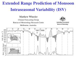
Madden-Julian Oscillation (MJO):30-60 days • Eastward propagating atmospheric disturbances associated to deep convection (see OLR above). • Bridge connecting diurnal and intraseasonal variability
MJO: Coupled Mode Composites of SST anomalies (contours) and OLR (colours) of MJO events. SST and convection are in quadrature. The lead-lag relationship between SST and deep convection seems instrumental for setting the propagation speed of the MJO. A two way coupling is required, but may not be enough. Thin ocean layers are needed to represent this phase relationship. See Frederic Vitart’spresentation.
Interannual Time scales: ENSO ENSO: El Nino -Southern Oscillation Largest mode of O-A interannual variability Best known source of predictability at seasonal time scales It affects global patterns of atmospheric circulation, with changes in rainfall, temperature, hurricans, extrem events • Main Characters: • Walker 1924, 1928 : Southern Oscillation Darwin-Tahiti • Peruvian fishermen: El Nino current interannualvariability • Bjerkness1966, 1969: EN-SO Coupled Ocean Atmosphere interaction and positive feedback • Wirtky 1975: Western Pacific Sea level as a predictor of El Nino (Kelvin wave propagation) • Philander 1990: A comprehensive book on ENSO • TAO array: Back-bone of the ENSO observing system
EL Nino (warm) and La Nina (cold) El Nino is associated with reduced easterly (maybe even westerly) winds at the surface, a reduced thermocline slope and warm water in the east. Normal/La Nina is associated with strong(er) easterly winds at the surface, a stronger thermocline tilt and cold water in the east.
Information from TAO-Moorings Anomaly Fields Zonal wind Thermocline Depth SST
Nino 3 Nino 3.4 WHERE ARE WE NOW? Sea Level Pressure (SOI) • In the equatorial Pacific, there is considerable interannual variability. • The EQSOI ( INDO-EPAC) is especially useful: it is a measure of pressure shifts in the tropical atmosphere but is more representative than the usual SOI (Darwin – Tahiti). • Note 1983, 87, 88, 97, 98 . Sea Surface Temperature (Nino 3)
El Nino Feedbacks: A complex Story From Philip et al 2010
Steps for seasonal Forecasts From J. Slingo, Royal Met Soc
Decadal: Pacific Decadal Oscillation • Considerable debate: Is it integrated red noise? Or a truly coupled mode? • Influences marine ecosystems (Mantua et al 1997), North American rainfall (Latif and Barnet 1994,1996, Waliser 2008) • Latif et al, using results from a coupled model, hypotesized there is a coupled feedback (SST-heat flux, gyre). Not confirmed by observations. • Latif et al: there is no need of a coupled mode nor ocean dynamics to produce decadal variability. • Link with ENSO decadal variability.
Atlantic Multidecadal Oscillation: AMO From King et al 2005 • Changes in the AMO linked to NE Brazil and Sahel rainfall, North Atlantic hurricane frequency, European and North American climate • Warm AMO phase during the 40-50’s associated to decreased NE Brazil rainfall, increased Sahel rainfall, increased hurricane frequency • Evidence from observations and model studies. • Is it connected to the AMOC (Atlantic Meridional Overturning circulation)?
Atlantic MOC Balmaseda et al 2007 Atlantic Variability and Climate Change Vellinga and Wood 2002: Surface Air Temperature change 20-30 years after the THC slowdown by large fresh water input. The THC recovers after 120 years Brydenet al 2005 suggested the slowing down of the AMOC based on 5 snapshots (red dots in figure). But large uncertainty due to possible aliasing RAPID program is monitoring the AMOC at 26N since 2004. But this is not long enough. Need of ocean re-analysis. But large uncertainty remains.
Summary of Coupled Ocean-Atmosphere Variability I • The ocean-atmosphere interaction can occur in a number of ways: • One way red noise • One way stochastic resonance • Two-ways coupled interaction • The kind of coupled interaction determines the predictability. • The nature of air sea interaction is very different in the tropics and in the extratropics. • In the tropics, the ocean drives the atmosphere: high values of SST can trigger deep convection. • The interaction occurs on a wide range of time scales: diurnal-interannual. • The representation of diurnal/intrasesonal variability needs fine vertical resolution in the ocean mixed layer. Mainly a thermodynamic response • The representation of the interannual variability, such as ENSO, needs the resolving the ocean below the thermocline and the dynamical response of the ocean to changes in the winds. • In the climate system all time scales are closely inter-related.