Download
1 / 49
500 likes | 741 Views
GIS and River Channels. By Venkatesh Merwade Center for Research in Water Resources, University of Texas, Austin. Instream flow studies. How do we quantify the impact of changing the naturalized flow of a river on species habitat?

E N D
GIS and River Channels By Venkatesh Merwade Center for Research in Water Resources, University of Texas, Austin
Instream flow studies • How do we quantify the impact of changing the naturalized flow of a river on species habitat? • How do we set the minimum reservoir releases that would satisfy the instream flow requirement?
Objective • Objective • To model species habitat as a function of flow conditions and help decision making • Instream Flow • Flow necessary to maintain habitat in natural channel.
Methodology • Species habitat are dependent on channel hydrodynamics – hydrodynamic modeling • Criteria to classify species depending on the conditions in the river channel – biological studies • Combine hydrodynamics and biological studies to make decisions – ArcGIS
Criterion Depth & velocity Species groups Habitat Hydrodynamic Habitat SMS/RMA2 Data Collection and some statistics Model Model Descriptions ArcGIS Instream Flow DecisionMaking Process Flowchart
Data Requirement • Hydrodynamic Modeling • Bathymetry Data (to define the channel bed) • Substrate Materials (to find the roughness) • Boundary Conditions (for hydrodynamic model) • Calibration Data (to check the model) • Biological Studies • Fish Sampling (for classification of different species) • Velocity and depth at sampling points
Study Area (Guadalupe river near Seguin, TX) 1/2 meter Digital Ortho Photography
Depth Sounder (Echo Sounder) The electronic depth sounder operates in a similar way to radar It sends out an electronic pulse which echoes back from the bed. The echo is timed electronically and transposed into a reading of the depth of water.
Acoustic Doppler Current Profiler Provides full profiles of water current speed and direction in the ocean, rivers, and lakes. Also used for discharge, scour and river bed topography.
Global Positioning System (GPS) Tells you where you are on the earth!
Final Setup GPS Antenna Computer and power setup Depth Sounder
Channel Movie A boat is moving along a River and bathymetry is recorded as set of points with (x,y,z) attributes.
Surface Water Modeling System (Environmental Modeling Systems, Inc.) RMA2 (US Army Corps of Engineers) 2D Hydrodynamic Model • SMS (Surface Water Modeling System) • RMA2 Interface • Input Data • Bathymetry Data • Substrate Materials • Boundary Conditions • Calibration Data
SMS mesh Finite element mesh and bathymetric data
Biological Studies (TAMU) • Meso Habitat and Micro Habitat • Use Vadas & Orth (1998) criterion for Meso Habitats • Electrofishing or seining to collect fish samples for Micro Habitat analysis • Sample at several flow rates and seasons • Measure Velocity and depth at seining points • Statistical analysis to get a table for Micro Habitats classification.
Deep Pool Run Depth [feet] Medium Pool Shallow Pool Fast Riffle Slow Riffle Mesohabitat Criteria: V, D, V/D, FR (Vadas & Orth, 1998)
Thalweg/Centerline Cross-sections ProfileLines Fishnet GIS database for river channels Measurement points Surface
Measure in ArcGIS A PolylineMZ can store m and z at each vertex along with x and y coordinates. 64.0056 0 112.3213
Defining a Thalweg Input Output Step 2 Step 1 Step 3 Step 4 User defines an arbitrary centerline over the measurement points Thalweg tool creates a surface using the measurement points Densify the initial centerline to get more points Normals are drawn at each vertex of the centerline to locate deepest points All the deepest points replace the vertices of the old centerline Final result is a 3D polyline defining the thalweg Old vertices New vertices
P s1 Centerlin e s2 n1 (s = 0, n = 0) n2 Bankline s P(n1, s1) Q(n2, s2) Q (s,n,z) coordinate system
n + o n - y n s n + x s o (x,y,z) n - s (s,n,z) (x,y,z) (s,n,z)
Surface in transformed coordiantes Straightened river Profile line and cross-sections Sinuous river
FishNet comparison Hydraulic FishNet Regular FishNet
Profile Lines and Cross Sections in 3D Bird’s eye view!
Courtesy: Texas Water Development Board • Priority segments are 100s of miles long • Representative reaches (study areas) are only a few (<5) miles long • Can we develop a channel description for the segments using the data for representative reaches?? • Useful not only for instream flows but also for other hydrologic studies
Some thoughts on blue lines • Blue lines on the hydrography map are pretty, but it would be nice if we know more about our river channels than just their location and shape • If we have the three-dimensional form of river channels then we can use it for preliminary studies and save lots of $$$
Thalweg location Cross-section form C C C C B B B B A A A A What do we know about river channels? Meandering shape
Methodology • We can get shape from the Blue lines • Using the shape we can locate the thalweg • Using the location of the thalweg, create cross-sections 3D form is not a problem, what about the dimensions?? They are different everywhere.. Work in a normalized domain where everything is Unity (one). We can re-scale the results using additional information..
@ 5 miles @ 30 miles Site1 and Site2 on Brazos River The data (bathymetry) for both sites is available as (x,y,z) points.
nL nR 0 - + Z P(ni, zi) d Zd w = nL + nR Normalizing the data For any point P(ni,zi), the normalized coordinates are: nnew = (ni – nL)/w znew = (Z – zi)/d For nL = -15, nR = 35, d = 5, Z=10 P (10, 7.5) becomesPnew(0.5, 0.5)
Normalized Data Original cross-section Modified cross-section Depth and width going from zero to unity makes life easier without changing the shape of the original cross-section
r1 r3 r2 Shape characterization through radius of curvature • Ifradius of curvature is small, the thalweg is close to the bank and as it increases the thalweg moves towards the center of the channel. • If the channel meanders to left, the center of curvature is to the right hand side of the centerline and vice versa. • When the center of curvature is to the right, the radius of curvature is considered positive and vice versa
Y = 0.076*log(x) + 1.21 Y = 0.087*log(x) – 0.32 Channel shape and thalweg 0 0.5 1.0
Thalweg and cross-section • Cross-section should have an analytical form to relate it to the thalweg • Many probability density functions (pdf) have shapes similar to the cross-section • Beta pdf is found feasible • its domain is from zero to one • it has only two parameters (a,b)
a < b a = b a > b real cross-sections (in red) are different especially at the tails beta probability density function Beta pdf looks good, but…..
Combination of two beta pdf beta c/s = (beta1 + beta2) * factor a1=5, b1=2, a2=3, b2=3, factor = 0.5 a1=2, b1=2, a2=3, b2=7, factor = 0.6
Thalweg location and beta Thalweg = 0.20 Thalweg = 0.40 a1=3.75, b1=5, a2 =1.75, b2 =1.75, f=0.25 a1=2.25, b1=7.5, a2 =2.25, b2 =2.25, f=0.225 a1=6, b1=3, a2 =2, b2 =2, f=0.24 Thalweg = 0.70
The final framework • If we start with a blue line, we can locate the thalweg using the relationship, t = f(s). • Using t, we can find the shape of cross-section using the relationship, c(a,b) = f(t). • The resulting cross-sections have a unit width and unit depth. • Rescale the normalized cross-sections using width (obtained from aerial photographs) and depth (hydraulic geometry)
Venkatesh Merwade Email: vmmerwade@mail.utexas.edu http://civilu.ce.utexas.edu/stu/merwadvm/