Download
1 / 197
1.97k likes | 2.1k Views
Macroeconomics 4. The Keynesian Model and its Policy Implications. Prof. Dr. Rainer Maurer. Macroeconomics. 4. The Keynesian Model and its Policy Implications 4.1. The Keynesian Theory 4.1.1. The "Keynesian Cross" 4.1.2. The Keynesian Model with Capital Market

E N D
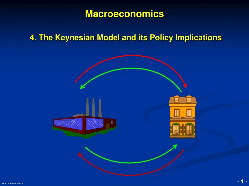
Macroeconomics4. The Keynesian Model anditsPolicyImplications Prof. Dr. Rainer Maurer
Macroeconomics 4. The Keynesian Model and its Policy Implications 4.1. The Keynesian Theory 4.1.1. The "Keynesian Cross" 4.1.2. The Keynesian Model with Capital Market 4.2. Demand-side Shocks 4.2.1. Reduction of the Propensity to Consume 4.2.2. Reduction of the Propensity to Invest 4.2.3. Consequences for the Labor Market 4.3. Fiscal and Monetary Policy in the Keynesian Model 4.3.1. Fiscal Policy 4.3.2. Monetary Policy 4.4. The Long-run Implications of the Keynesian Model 4.5. Policy Conclusions 4.5.1. Practical Problems of Anti-cyclical Policy 4.5.2. Case Study: Fiscal Policy in Germany 4.5.3. Limits of Government Debt 4.5.4. Case Study: Economic Policy in the Great Recession 4.6. Questions for Review Prof. Dr. Rainer Maurer
Macroeconomics Literature: ◆ Chapter 9, 10, 11, 13, 14 Mankiw, Gregory; Macroeconomics, Worth Publishers. ◆ Kapitel 10, Baßeler, Ulrich et al.; Grundlagen u. Probleme der Volkswirtschaft, Schäfer-Pöschel. Prof. Dr. Rainer Maurer - 3 -
Macroeconomics 4. The Keynesian Model and its Policy Implications 4.1. The Keynesian Theory Prof. Dr. Rainer Maurer - 4 -
4. The Keynesian Model anditsPolicyImplications4.1. The KeynesianTheory The Crisis of Neoclassical Theory Until the world economic crisis of 1929, the neoclassical model was the consensus model of market oriented economists. This appraisal of the neoclassical theory was altered by the world economic crisis. Such a sharp and lasting break of economic development was inconsistentwith the neoclassical hypothesis of the immanent stability of market economies. Rising unemployment, bankrupt companies and decreasing incomes caused social problems that calledfor new solutions. Prof. Dr. Rainer Maurer - 5 -
4. The Keynesian Model anditsPolicyImplications4.1. The KeynesianTheory The Development of the Dow Jones Index Prof. Dr. Rainer Maurer - 7 - Quelle: www.dowjones.com
4. The Keynesian Model anditsPolicyImplications4.1. The KeynesianTheory Prof. Dr. Rainer Maurer - 8 -
4. The Keynesian Model anditsPolicyImplications4.1. The KeynesianTheory The analysis of demand shocks in the neoclassical model has revealed that a reduction of consumption demand should lead to an increase in savings, which should reduce the interest rate such that demand for investment goods grows and replace the reduction in consumption (and vice versa). This mechanism did not work in the world economic crisis! Prof. Dr. Rainer Maurer - 9 -
4. The Keynesian Model anditsPolicyImplications4.1. The KeynesianTheory The Keynesian Theory Under these historical circumstances John Maynard Keynes developed his new macroeconomic theory, which was intended to explain the consequences of the world economic crisis and to deliver economic policy recommendations appropriate to overcome such a crisis. This theory was published in a book with the title “General Theory of Employment, Interest and Money” (1936). In this book, Keynes contested two basic assumptions of the neoclassical theory by assuming that …in the short run, goods prices are fix, so that they cannot de-crease in case of a reduction of goods demand. As a consequen-ce, he assumed that instead of goods prices the supply of goods adjusts to changes in demand = “Keynesian Price Rigidity”. …household consumption is only a positive function of household income C(Y ↑)↑; the negative impact of the interest rate C(i↓)↑ can be neglected = “Keynesian Consumption Function”. Prof. Dr. Rainer Maurer - 13 -
4. The Keynesian Model anditsPolicyImplications4.1. The KeynesianTheory The Keynesian consumption function C(Y↑)↑ corresponds at first sight much better to empirical observations as the neoclassical consumption function C(i↑)↓. The empirical correlation between consumption and income is in deed much stronger than the empirical correlation between consumption and interest rates, as the following graphs demonstrate: Prof. Dr. Rainer Maurer - 14 -
= C(Y↑)↑ = Keynesian Consumption Function Prof. Dr. Rainer Maurer - 15 - Quelle: SVG (2003), eigene Berechnungen
= C(i↑)↓ = Neoclassical Consumption Function Quelle: SVG (2003), eigene Berechnungen Prof. Dr. Rainer Maurer - 16 -
4. The Keynesian Model anditsPolicyImplications4.1. The KeynesianTheory The second basic difference between Keynesian and neo-classical theory is the so called “Keynesian Price Rigidity”: In neoclassical theory, an increase of production output causes an increase of marginal costs, so that firms increase their prices (and vice versa). Consequently, an increase of the demand for goods causes an increase of the prices of goods (and vice versa). In Keynesian theory, firms do not immediately adjust their prices to production output: An increase (decrease) of the demand for goods causes a corresponding increase (decrease) of the supply of goods. The prices of goods stay however constant. Who is right – Keynes or the Neoclassics? Prof. Dr. Rainer Maurer - 17 -
4. The Keynesian Model anditsPolicyImplications4.1. The KeynesianTheory p S(p)1 S(p)1 Production costs higher than market price Price increase with time lag p1 p1 D(p)2 D(p)2 D(p)1 D(p)1 Immediate increase of production Neoclassical Market Keynesian Market Prof. Dr. Rainer Maurer - 18 -
An large-scale empirical study of the European Central Bank has led to the following result: 4. The Keynesian Model anditsPolicyImplications4.1. The KeynesianTheory Percentage Distribution of Firms According Their Frequency of Price Adjustments per Year Survey Period 2003-2004; Sample Size 11000 Firms; BE = Belgium, DE= Germany; FR=France, IT=Italy LU= Luxembourg, NL=Netherlands, AT=Austria, PT=Portugal - 19 - Prof. Dr. Rainer Maurer Quelle: The Pricing Behavior of Firms in the Euro Area, EZB (2005)
4. The Keynesian Model anditsPolicyImplications4.1. The KeynesianTheory From these and similar studies follows: Firms do not immediately adjust their prices to changes in costs. Instead, they keep their prices constant over a longer period of time – just as assumed by Keynes. If firms try to maximize their profits, they should in principle change their prices when their costs change. Why then do firms not change their prices more often? Prof. Dr. Rainer Maurer - 21 -
4. The Keynesian Model anditsPolicyImplications4.1. The KeynesianTheory Why do prices not change more often? In reality, changing prices causes costs: Internal organizational costs: Information of staff members, distribution chains, sales agents… External communication costs: Explication and justification of price changes to clients… Technical costs: printing costs of pricelists, mailing expenses… If the costs per price change are higherthan the return of a price change, a continuous adjustment of prices is not profit maximizing, as the following diagram shows: Prof. Dr. Rainer Maurer - 22 -
4. The Keynesian Model anditsPolicyImplications4.1. The KeynesianTheory € The costs per price change will typically be constant or slightly increasing, if the number of price changes per year grows. Costs per Price Change 3 € 3 € Number of Price Changes per Year 5,5 3,0 3,5 0,5 1,0 2,0 6,0 2,5 4,0 4,5 5,0 1,5
4. The Keynesian Model anditsPolicyImplications4.1. The KeynesianTheory € The costs per price change will typically be constant or slightly increasing, if the number of price changes per year grows. Costs per Price Change 3 € 6 € Number of Price Changes per Year 5,5 3,0 3,5 0,5 1,0 2,0 6,0 2,5 4,0 4,5 5,0 1,5
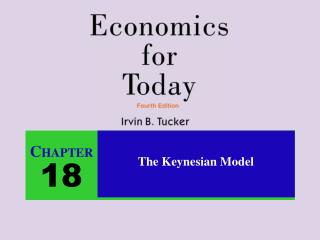
4. The Keynesian Model anditsPolicyImplications4.1. The KeynesianTheory € The return per price change will typically decrease, if the number of price changes per year grows. The return of 1 price change every 2 years will normally be quite high, since it is very likely that significant changes of production costs and demand strength will occur within a time span of 2 years. The return of 4 price changes per year will normally be lower, since it is not so likely that significant chan-ges of production costs and demand strength will occur every quarter… Return per Price Change Number of Price Changes per Year 5,5 3,0 3,5 0,5 1,0 2,0 6,0 2,5 4,0 4,5 5,0 1,5
4. The Keynesian Model anditsPolicyImplications4.1. The KeynesianTheory € Return of an additional price change higher than costs Costs per Price Change Return per Price Change More often price changes profitable Number of Price Changes per Year 5,5 3,0 3,5 0,5 1,0 2,0 6,0 2,5 4,0 4,5 5,0 1,5
4. The Keynesian Model anditsPolicyImplications4.1. The KeynesianTheory € Return of an additional price change lower than costs Costs per Price Change Return per Price Change Less often price change profitable Number of Price Changes per Year 5,5 3,0 3,5 0,5 1,0 2,0 6,0 2,5 4,0 4,5 5,0 1,5
4. The Keynesian Model anditsPolicyImplications4.1. The KeynesianTheory € => Profit maximizing number of price changes per year = 2 Costs per Price Change Return per Price Change Number of Price Changes per Year 5,5 3,0 3,5 0,5 1,0 2,0 6,0 2,5 4,0 4,5 5,0 1,5
4. The Keynesian Model anditsPolicyImplications4.1. The KeynesianTheory € Profit at 2 adjustments of prices per year => Profit maximizing number of price changes per year = 2 Costs per Price Change Return per Price Change Number of Price Changes per Year 5,5 3,0 3,5 0,5 1,0 2,0 6,0 2,5 4,0 4,5 5,0 1,5
4. The Keynesian Model anditsPolicyImplications4.1. The KeynesianTheory € => The higher the costs per price adjustment, the lower the number of profit maximizing price adjustments per year! Costs per Price Change2 Costs per Price Change1 Return per Price Change Number of Price Changes per Year 5,5 3,0 3,5 0,5 1,0 2,0 6,0 2,5 4,0 4,5 5,0 1,5
4. The Keynesian Model anditsPolicyImplications4.1. The KeynesianTheory As the diagrams show: It is possible to explain, why firms on average do not change their prices more often than one time per year with the standard microeconomic profit-maximization behavior: An optimal adjustment of prices according to the current demand and supply situation causes an additional return. But this return has to be compared to the additional costs caused by the price adjustment. Only if the additional return is larger than the additional costs, a price adjustment is actually profitable. Depending on the relationbetween the costs and returnof a price change it can be profit-maximizing to hold prices on average constant for a time span of a year or even longer. Rigid price setting and profit maximization are compatible! Prof. Dr. Rainer Maurer - 33 -
4. The Keynesian Model anditsPolicyImplications4.1. The KeynesianTheory The Keynesian theory assumes therefore that in the “short-run” (= within a time span of one year) firms keep their prices constant: P = constant within one year If the demand for goods changes in the short-run, firms do simply adjust their production instead of prices to the demand for goods. Consequently, in the short-run firms' production of goods Y is always equal to the sum of households consumption demandC plus firms’ demand for investment goods I plus government consumption demand G: Y = C + I + G Consequently, in the short-run demand for goods determines supply of goods! Prof. Dr. Rainer Maurer - 34 -
4. The Keynesian Model anditsPolicyImplications4.1. The KeynesianTheory If we add now the Keynesian consumption function C(Y) we receive the following relationship: Y = C(Y) + I + G Obviously, this is a circular relationship: GDP, Y, depends on consumption C(Y) and consumption C(Y) depends on GDP Y and so on… As the following analysis will show, this circular relationship can boost the effects of economic policy (but complicates a bit the graphical analysis…). Prof. Dr. Rainer Maurer - 35 -
Macroeconomics 4. The Keynesian Model and its Policy Implications 4.1. The Keynesian Theory 4.1.1. The "Keynesian Cross" Prof. Dr. Rainer Maurer - 36 -
4. The Keynesian Model and its Policy Implications4.1.1. The "Keynesian Cross" Demand for Goods Graphical exposition of these considerations: C(Y)= 0,5 * Y Supply of Goods = Production of Goods = Income = Y Prof. Dr. Rainer Maurer - 43 -
4. The Keynesian Model anditsPolicyImplications4.1.1. The "Keynesian Cross" Demand for Goods Consumption (C) dependent on GDP (Y) C(Y)= 0,5 * Y Supply of Goods = Production of Goods = Income = Y Prof. Dr. Rainer Maurer - 44 -
4. The Keynesian Model anditsPolicyImplications4.1.1. The "Keynesian Cross" Demand for Goods C(Y) + G = 0,5*Y+G C(Y)= 0,5 * Y Government Consumption = G = 5 Supply of Goods = Production of Goods = Income = Y Prof. Dr. Rainer Maurer - 45 -
4. The Keynesian Model anditsPolicyImplications4.1.1. The "Keynesian Cross" Demand for Goods YD = 0,5*Y+G+I C(Y) + G = 0,5*Y+G Investment = I = 5 C(Y)= 0,5 * Y Supply of Goods = Production of Goods = Income = Y Prof. Dr. Rainer Maurer - 46 -
4. The Keynesian Model and its Policy Implications4.1.1. The "Keynesian Cross" Demand for Goods At what level of income (Y) does the total demand for goods equalincome? YD = 0,5*Y+G+I C(Y) + G = 0,5*Y+G C(Y) = 0,5 * Y At what level does income generate a demandfor goods, which is again equal to the level of income? = Where does the equation 0,5*Y+G+I = Y hold? Supply of Goods = Production of Goods = Income = Y Prof. Dr. Rainer Maurer - 47 -
4. The Keynesian Model anditsPolicyImplications4.1.1. The "Keynesian Cross" Demand for Goods Every point on this 45°-line implies: Demand for Goods = Supply of Goods Supply of Goods = Production of Goods = Income = Y Prof. Dr. Rainer Maurer - 48 -
4. The Keynesian Model anditsPolicyImplications4.1.1. The "Keynesian Cross" Demand for Goods The 45°-line reveals the solution: YD = 0,5*Y+G+I C(Y) + G = 0,5*Y+G C(Y)= 0,5 * Y Supply of Goods = Production of Goods = Income = Y Prof. Dr. Rainer Maurer - 49 -
4. The Keynesian Model anditsPolicyImplications4.1.1. The "Keynesian Cross" Demand for Goods YD = 0,5*Y+G+I C(Y) + G = 0,5*Y+G C(Y)= 0,5 * Y Investment = 5 Gov. Consumption = 5 Consumption = 0,5 * (20) = 10 Supply of Goods = Production of Goods = Income = Y Prof. Dr. Rainer Maurer - 50 -
3. Das keynesianische Modell der Volkswirtschaft3.1. Die Struktur des keynesianischen Modells Digression: What happens, if supply of goods is larger than the equilibrium value = if there is excess supply ? The following digression shows that in this case an adjustment process takes place. Since supply of goods under Keynesian assumptions always adjusts to demand for goods, supply falls until it equals demand: Prof. Dr. Rainer Maurer - 51 - F49-F66
3. Das keynesianische Modell der Volkswirtschaft3.1. Die Struktur des keynesianischen Modells Digression: What happens, if supply of goods is smaller than the equilibrium value = if there is excess demand ? The following digression shows that in this case an adjustment process takes place. Since supply of goods under Keynesian assumptions always adjusts to demand for goods, supply grows until it equals demand: Prof. Dr. Rainer Maurer - 61 -
4. The Keynesian Model anditsPolicyImplications4.1. The KeynesianTheory What happens now, if the equilibrium on the market for goods is disturbed by a sudden increase in investment demand? Prof. Dr. Rainer Maurer - 68 -
4. The Keynesian Model anditsPolicyImplications4.1.1. The "Keynesian Cross" Demand for Goods YD = 0,5*Y+G+I C(Y) + G = 0,5*Y+G C(Y)= 0,5 * Y How strong is GDP-growth, if investment grows by 5 ? Supply of Goods= Income = Y Prof. Dr. Rainer Maurer - 69 -
4. The Keynesian Model anditsPolicyImplications4.1.1. The "Keynesian Cross" Increase in Invest-ment by 5 Demand for Goods YD= 0,5*Y+G+I+ΔI YD = 0,5*Y+G+I C(Y) + G = 0,5*Y+G C(Y)= 0,5 * Y How strong is GDP-growth, if investment grows by 5 ? Supply of Goods= Income = Y Prof. Dr. Rainer Maurer - 70 -
4. The Keynesian Model and its Policy Implications4.1.1. The "Keynesian Cross" Demand for Goods YD= 0,5*Y+G+I+ΔI YD = 0,5*Y+G+I C(Y) + G = 0,5*Y+G C(Y)= 0,5 * Y Increase in Invest-ment by 5 Increase in GDP by 10 = 5 * (1/(1-0,5)) Supply of Goods= Income = Y Prof. Dr. Rainer Maurer - 71 -
4. The Keynesian Model anditsPolicyImplications4.1.1. The "Keynesian Cross" Demand for Goods YD= 0,5*Y+G+I+ΔI YD = 0,5*Y+G+I Investment = 10 C(Y) + G = 0,5*Y+G C(Y)= 0,5 * Y Gov. Consumption = 5 Increase in invest-ment by 5 Growth of Consumption = 5 Consumption = 0,5*20 = 10 Consumption = 0,5 * 30 = 15 Supply of Goods= Income = Y Prof. Dr. Rainer Maurer - 72 -
4. The Keynesian Model anditsPolicyImplications4.1.1. The "Keynesian Cross" Demand for Goods YD= 0,5*Y+G+I+ΔI YD = 0,5*Y+G+I C(Y) + G = 0,5*Y+G C(Y)= 0,5 * Y As implied by the investment multiplier 1/(1-c), a consumption ratio of c = 50% together with an increase in investment by 5 causes GDP to grow by 10 = 5 * (1/(1-0,5)) = 5 * 2. Increase in Invest-ment by 5 Supply of Goods= Income = Y Prof. Dr. Rainer Maurer - 73 -
4. The Keynesian Model anditsPolicyImplications4.1. The KeynesianTheory The following diagram graphically illustrates the multiplier effect: Prof. Dr. Rainer Maurer - 74 -
4. The Keynesian Model and its Policy Implications4.1.1. The "Keynesian Cross" YD= 0,5*Y+G+I+ΔI Demand for Goods YD = 0,5*Y+G+I 1st: Increase in Demand by 5 C(Y) + G = 0,5*Y+G C(Y)= 0,5 * Y Increase in Invest-ment by 5 What causes the multiplier effect? Supply of Goods= Income = Y Prof. Dr. Rainer Maurer - 75 -
4. The Keynesian Model anditsPolicyImplications4.1.1. The "Keynesian Cross" YD= 0,5*Y+G+I+ΔI Demand for Goods YD = 0,5*Y+G+I C(Y) + G = 0,5*Y+G 2nd: Increase in Income by 5 = ΔY C(Y)= 0,5 * Y Increase in Invest-ment by 5 What causes the multiplier effect? Supply of Goods= Income = Y Prof. Dr. Rainer Maurer - 76 -
4. The Keynesian Model anditsPolicyImplications4.1.1. The "Keynesian Cross" YD= 0,5*Y+G+I+ΔI Demand for Goods YD = 0,5*Y+G+I 3rd: Increase in Consumption by c*ΔY = 0,5 * 5 = 2,5 C(Y) + G = 0,5*Y+G C(Y)= 0,5 * Y Increase in Invest-ment by 5 What causes the multiplier effect? Supply of Goods= Income = Y Prof. Dr. Rainer Maurer - 77 -
4. The Keynesian Model anditsPolicyImplications4.1.1. The "Keynesian Cross" YD= 0,5*Y+G+I+ΔI Demand for Goods YD = 0,5*Y+G+I C(Y-T) + G C(Y)= 0,5*Y+G 4th: Increase in Income by ΔY = 2,5 C(Y)= 0,5 * Y Increase in Invest-ment by 5 What causes the multiplier effect? Supply of Goods= Income = Y Prof. Dr. Rainer Maurer - 78 -