Download
1 / 26
260 likes | 394 Views
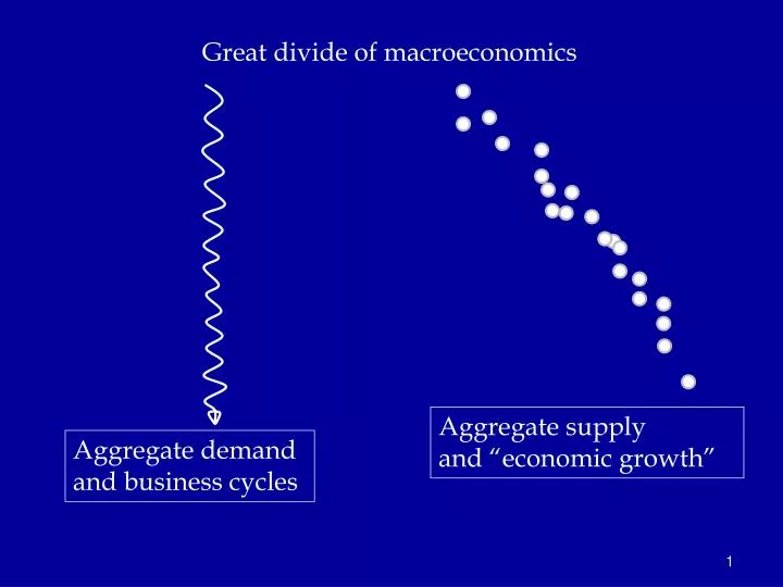
Great divide of macroeconomics. Aggregate supply and “economic growth”. Aggregate demand and business cycles. The Great Divide. Classical macro: - Full employment - Flexible wages and prices - Perfect competition and rational expectations

E N D
Great divide of macroeconomics Aggregate supply and “economic growth” Aggregate demand and business cycles
The Great Divide Classical macro: - Full employment - Flexible wages and prices - Perfect competition and rational expectations - Only “real” business cycles, and all unemployment is voluntary and efficient Keynesian macro: - Underutilized resources - Inflexible (or fixed) wages and prices - Imperfect competition and behavioral expectations - Yes, business cycles, with persistent slumps, involuntary unemployment, and macro waste.
Understanding business cycles Major elements of cycles • short-period (1-3 yr) erratic fluctuations in output • pro-cyclical movements of employment, profits, prices • counter-cyclical movements in unemployment • appearance of “involuntary” unemployment in recessions Historical trends • lower volatility of output, inflation over time (until 2008) • movement from stable prices to rising prices since WW II
The incomplete recovery Full employment Shaded areas are NBER recessions.
Output gaps and the business cycle Large GDP “gap”
“The Great Moderation on Output” GOLD STANDARD Definition of volatility (often used in finance): the standard deviation of returns or rates of growth, usually at an annual rate.
“The Great Moderation on Inflation” GOLD STANDARD
IS-MP model The major tool for showing the impact of monetary and fiscal polices, along with the effect of various shocks, in a short-run Keynesian situation. The “MP” function replaces the “LM” function, which is obsolete. Check the reading list very carefully! Key assumptions in short-run macro model: • Fixed prices (P=1 and π = 0); or can have fixed inflation. • Unemployed resources (Y < potential Y = Mankiw’s natural Y) • Closed economy (inessential and considered later) • Goods markets (IS) and financial markets (MP)
IS curve (expenditures) Basic idea: describes equilibrium in goods market. Finds Y where planned I = planned S or planned expenditure = planned output. Basic set of equations: • Y = C + I + G • C = a + b(Y-T) • T = T0 + τ Y [note assume income tax, τ = marginal tax rate] • I = I0 – dr [note i = r because zero inflation] • G = G0
which gives the IS curve: (IS) Y =a - bT0 + G0 + I0 - dr 1 - b(1- τ) (IS) Y = μ [A0 - dr] where A0 = autonomous spending = a - bT0 + G0 + I0 μ = simple Keynesian multiplier = 1/[(1 - b(1- τ)] which we graph as the IS curve. Note that changes in fiscal policy, investment “animal spirits,” consumption wealth effect SHIFT IS CURVE HORIZONTALLY.
IS curve r = real interest rate IS(G, T0, …) Y = real output (GDP)
IS curve r = real interest rate IS(G’, T0, …) IS(G, T0, …) Y = real output (GDP)
MP curve (monetary policy/financial markets) The simplest MP curve says that the Fed sets the short term interest rate (i). With given inflation, this gives real interest rate: So with Fed setting the interest rate, this is simple MP curve: (MP) r = i - π
IS-MP diagram r = real interest rate E MP(π*) re IS(G, T0, …) Ye Y = real output (GDP)
… to the real stuff • In reality, the Fed has a “dual mandate”(see below). • This is usually represented by the Taylor rule, so let’s go there.
The Dual Mandate Fed’s dual mandate (Federal Reserve Act as amended): “promote effectively the goals of maximum employment, stable prices and moderate long-term interest rates.” In practice (FOMC statement January 2012): “The Committee judges that inflation at the rate of 2 percent, as measured by the annual change in the price index for personal consumption expenditures, is most consistent over the longer run with the Federal Reserve's statutory mandate.” “The maximum level of employment is largely determined by nonmonetary factors that affect the structure and dynamics of the labor market…In the most recent projections, FOMC participants' estimates of the longer-run normal rate of unemployment had a central tendency of 5.2 percent to 6.0 percent”
MP curve with the dual mandate The Taylor Rule Begin with a monetary policy equation in the form of a “Taylor rule”: (TR) i = π + r* + b(π-π*) + cy r* is the equilibrium real interest rate, π inflation rate, π* is inflation target, y is log output gap [log(Y/Yp)], b and c are parameters.
MP curve with the dual mandate The Taylor Rule Begin with a monetary policy equation in the form of a “Taylor rule”: (TR) i = π + r* + b(π-π*) + cy r* is the equilibrium real interest rate, π inflation rate, π* is inflation target, y is log output gap [log(Y/Yp)], b and c are parameters. 2. Assume for now that inflation is at target. So π = π* and we have financial market: (MP) r = r* + cy Later on, we will introduce inflation.
MP curve with inflation Now add inflation to the MP curve. Assume that inflation is a function of output (this will be done later): (PC)π= π*+φ y + η (η=inflation shock) (TR) i = π + r* + b(π-π*) + cy So new MP curve is: i = π + r* + b(φ y + η) + cy or (MP) i = π + r* + (bφ+c) y + bη So adding inflation makes the MP curve steeper, but does not change the basic structure..
Algebra of IS-MP Analysis • The analysis looks at simultaneous equilibrium in goods market and financial markets (Main St and Wall St). • The algebraic solution for equilibrium Ye is: Ye = μ*A0 –μ* d r* where μ* = μ/(1 + μdc) = multiplier with monetary policy. μ= simple multiplier > μ* ; A0 = autonomous spending = a - bT0 + G0 + I0 , Note impacts on output: Positive: G, I0, NX Negative: risk premium (and later inflation shock)
IS-MP diagram r = real interest rate MP(r*) E re IS(G, T0, …) Ye Y = real output (GDP)
1. What are the effects of fiscal policy? • A fiscal policy is change in purchases (G) or in taxes (T0,τ), holding monetary policy constant. • In normal times, because MP curve slopes upward, expenditure multiplier is reduced due to crowding out.
IS shock (as in fiscal expansion) MP i IS(G’) IS(G) Y = real output (GDP)
Multiplier Estimates by the CBO Congressional Budget Office, Estimated Impact of the ARRA, April 2010
MP(ηt > 0) Inflationary shock MP(ηt = 0) i it** IS Yt** Y = real output (GDP)