Download
1 / 37
410 likes | 570 Views
Bayesian AVO Inversion and Application to a Case Study. P ål Dahle * , Ragnar Hauge, and Od d Kolbjørnsen Norwegian Computing Center Nam H. Pham Statoil. Contents. Objective Constrain high resolution 3D reservoirs by seismic AVO data Method

E N D
Bayesian AVO Inversion and Application to a Case Study Pål Dahle*, Ragnar Hauge, and Odd Kolbjørnsen Norwegian Computing Center Nam H. Pham Statoil
Contents Objective • Constrain high resolution 3D reservoirs by seismic AVO data Method • Bayesian inversion, merging of geophysical and geological models Contribution • Fast algorithm • Spatial coupling • Uncertainty assessment Vp Vs
Outline 1) Geophysical model Bayesian inversion 2) Earth model 3) Combining models Combined 4) Summary Geology 5) Case study Rapid spatially coupled AVO inversion Probability Seismic Reservoir
Convolutional model: d(x,t,) = wtcpp(x,t,) + (x,t,) * d(x,t,) AVO-trace, surface point x, “offset” w (t)Seismic wavelet, angle dependentcpp(x,t,) Seismic reflectivity(x,t,) Error term w (t) cpp(x,t,) d(x,t,) Geophysical Model
Weak contrast approximation (continuous version): Convolutional model: m(x,t) = [ lnVp(x,t), lnVs(x,t), ln(x,t) ] d(x,t,) = wtcpp(x,t,) + (x,t,) * cpp(x,t,) = aVp() lnVp(x,t)+ aVs() lnVs(x,t) + a() ln(x,t) t t t Reflectivity Matrix formulation:d = Gm +
m(x,t) = [ lnVp(x,t), lnVs(x,t), ln(x,t) ] m ~ N( m,m) ~ N(0,e) d~ N( md,d) Assuming Normal Distributions Matrix formulation:d = Gm +
m= CovmH (x1,t1), mH (x2,t2) Earth Model Vp Isotropic, inhomogeneous earth: m(x,t) = mBG(x,t)+mH(x,t) Vs m ~ N(mBG,m)
CovmH (x1,t1), mH (x2,t2) =0(t1 - t2 ) (x1 - x2 ) ln lnVs ln 7.6 7.80 7.80 7.4 7.75 7.75 7.2 7.70 7.70 7.0 7.8 7.9 8.0 7.8 7.9 8.0 7.2 7.4 7.0 lnVp lnVp lnVs m: Inter-parameter Dependence
CovmH (x1,t1), mH (x2,t2) =0(t1 - t2 ) (x1 - x2 ) m: Vertical Dependence Vp 2100 1 2200 0 -20 0 20 2300 2000 2500 3000
CovmH (x1,t1), mH (x2,t2) =0(t1 - t2 ) (x1 - x2 ) 1350 1350 1 1300 1250 1250 0 40 -40 0 0 -40 40 1500 1600 1700 m: Lateral Dependence Vp
m ~ N( m,m) ~ N(0,e) d~ N( md,d) m d ~ N( mm|d , m|d) Combining the Models
mm|d = mBG+mG*(GmG* + e)-1(d - GmBG) m|d = m - mG*(GmG* + e)-1G m m,d m d The Posterior Distribution too much time ....
m,d m d 3D FFT 3D inverse FFT m,d m d Solving in Frequency Space
Summary • Bayesian inversion • Convolutional model,weak contrast • Spatial dependencies of earth parameters • Fast inversion • 100 million grid cells ~ 1 hour • More than inversion • Consistent merging of well logs • High resolution reservoirs
The Smørbukk Case • 32 mill grid cells • 3 angles • 2.5 h
Frequency Split • Background freq < 6Hz • Inversion 6Hz ≤ freq ≤ 40Hz • Simulation freq > 40Hz
Background Model Vp6 Vs6 RHOB6
Inversion Input Data • Background model: Vp, Vs, and Rho • Well data: TWT, DT, DTS, and Rho • Seismic Data • Wavelets
AI Prediction in Wells Well 1Well 2Well 3
SI Prediction in Wells Well 1Well 2Well 3
Density Prediction in Wells Well 1Well 2Well 3
AI Background Well
AI Prediction Well
AI Prediction Conditioned to Wells Well well
Case Study Conclusions • Good match for AI used for modelling of • Facies • Porosity