Download
1 / 28
590 likes | 1.8k Views
3D Sensing. Camera Model and 3D Transformations Camera Calibration (Tsai’s Method) Depth from General Stereo (overview) Pose Estimation from 2D Images (skip) 3D Reconstruction. Camera Model: Recall there are 5 Different Frames of Reference. yc. xc. Object World Camera

E N D
3D Sensing • Camera Model and 3D Transformations • Camera Calibration (Tsai’s Method) • Depth from General Stereo (overview) • Pose Estimation from 2D Images (skip) • 3D Reconstruction
Camera Model: Recall there are 5 Different Frames of Reference yc xc • Object • World • Camera • Real Image • Pixel Image zw yf C xf image a W zc yw pyramid object zp A yp xp xw
Rigid Body Transformations in 3D zp pyramid model in its own model space zw xp W yp rotate translate scale yw instance of the object in the world xw
Rotation in 3D is about an axis z rotation by angle about the x axis y x Px Py Pz 1 1 0 0 0 0 cos - sin 0 0 sin cos 0 0 0 0 1 Px´ Py´ Pz´ 1 =
Rotation about Arbitrary Axis R1 R2 T One translation and two rotations to line it up with a major axis. Now rotate it about that axis. Then apply the reverse transformations (R2, R1, T) to move it back. Px´ Py´ Pz´ 1 Px Py Pz 1 r11 r12 r13 tx r21 r22 r23 ty r31 r32 r33 tz 0 0 0 1 =
The Camera Model How do we get an image point IP from a world point P? Px Py Pz 1 c11 c12 c13 c14 c21 c22 c23 c24 c31 c32 c33 1 s Ipr s Ipc s = image point world point camera matrix C What’s in C?
The camera model handles the rigid body transformation from world coordinates to camera coordinates plus the perspective transformation to image coordinates. 1. CP = T R WP 2. IP = (f) CP CPx CPy CPz 1 s Ipx s Ipy s 1 0 0 0 0 1 0 0 0 0 1/f 1 = image point perspective transformation 3D point in camera coordinates
Camera Calibration • In order work in 3D, we need to know the parameters • of the particular camera setup. • Solving for the camera parameters is called calibration. yc • intrinsic parameters are • of the camera device • extrinsic parameters are • where the camera sits • in the world yw xc C zc W xw zw
Intrinsic Parameters • principal point (u0,v0) • scale factors (dx,dy) • aspect ratio distortion factor • focal length f • lens distortion factor • (models radial lens distortion) C f (u0,v0)
Extrinsic Parameters • translation parameters • t = [tx ty tz] • rotation matrix r11 r12 r13 0 r21 r22 r23 0 r31 r32 r330 0 0 0 1 R = Are there really nine parameters?
Calibration Object The idea is to snap images at different depths and get a lot of 2D-3D point correspondences.
The Tsai Procedure • The Tsai procedure was developed by Roger Tsai • at IBM Research and is most widely used. • Several images are taken of the calibration object • yielding point correspondences at different distances. • Tsai’s algorithm requires n > 5 correspondences • {(xi, yi, zi), (ui, vi)) | i = 1,…,n} • between (real) image points and 3D points.
In this* version of Tsai’s algorithm, • The real-valued (u,v) are computed from their pixel • positions (r,c): • u = dx (c-u0) v = -dy (r - v0) • where • - (u0,v0) is the center of the image • - dx and dy are the center-to-center (real) distances • between pixels and come from the camera’s specs • - is a scale factor learned from previous trials * This version is for single-plane calibration.
Tsai’s Geometric Setup Oc y camera x image plane principal point p0 pi = (ui,vi) y (0,0,zi) Pi = (xi,yi,zi) x 3D point z
Tsai’s Procedure 1. Given the n point correspondences ((xi,yi,zi), (ui,vi)) Compute matrix A with rows ai ai = (vi*xi, vi*yi, -ui*xi, -ui*vi, vi) These are known quantities which will be used to solve for intermediate values, which will then be used to solve for the parameters sought.
Intermediate Unknowns 2. The vector of unknowns is = (1, 2, 3, 4, 5): 1=r11/ty 2=r12/ty 3=r21/ty 4=r22/ty 5=tx/ty where the r’s and t’s are unknown rotation and translation parameters. 3. Let vector b = (u1,u2,…,un) contain the u image coordinates. 4. Solve the system of linear equations A = b for unknown parameter vector .
Use to solve for ty, tx, and 4 rotation parameters 2 2 2 2 2 5. Let U = 1 + 2 + 3 + 4 . Use U to calculate ty .
6. Try the positive square root ty = (ty ) and use it to compute translation and rotation parameters. 1/2 2 r11 = 1 ty r12 = 2 ty r21 = 3 ty r22 = 4 ty tx = 5 ty Now we know 2 translation parameters and 4 rotation parameters. except…
Determine true sign of ty and computeremaining rotation parameters. 7. Select an object point P whose image coordinates (u,v) are far from the image center. 8. Use P’s coordinates and the translation and rotation parameters so far to estimate the image point that corresponds to P. If its coordinates have the same signs as (u,v), then keep ty, else negate it. 9. Use the first 4 rotation parameters to calculate the remaining 5.
Solve another linear system. 10. We have tx and ty and the 9 rotation parameters. Next step is to find tz and f. Form a matrix A´ whose rows are: ai´ = (r21*xi + r22*yi + ty, vi) and a vector b´ whose rows are: bi´ = (r31*xi + r32*yi) * vi 11. Solve A´*v = b´ for v = (f, tz).
Almost there 12. If f is negative, change signs (see text). 13. Compute the lens distortion factor and improve the estimates for f and tz by solving a nonlinear system of equations by a nonlinear regression. 14. All parameters have been computed. Use them in 3D data acquisition systems.
We use them for general stereo. P y1 y2 P2=(r2,c2) x2 P1=(r1,c1) e2 e1 x1 C1 C2
For a correspondence (r1,c1) inimage 1 to (r2,c2) in image 2: 1. Both cameras were calibrated. Both camera matrices are then known. From the two camera equations we get 4 linear equations in 3 unknowns. r1 = (b11 - b31*r1)x + (b12 - b32*r1)y+ (b13-b33*r1)z c1 = (b21 - b31*c1)x + (b22 - b32*c1)y + (b23-b33*c1)z r2 = (c11 - c31*r2)x+ (c12 - c32*r2)y+ (c13 - c33*r2)z c2 = (c21 - c31*c2)x+ (c22 - c32*c2)y + (c23 - c33*c2)z Direct solution uses 3 equations, won’t give reliable results.
Solve by computing the closestapproach of the two skew rays. P1 If the rays intersected perfectly in 3D, the intersection would be P. solve for shortest V P Q1 Instead, we solve for the shortest line segment connecting the two rays and let P be its midpoint.
Application: Kari Pulli’s Reconstruction of 3D Objects from light-striping stereo.
Application: Zhenrong Qian’s 3D Blood Vessel Reconstruction from Visible Human Data