Consumer Price Index

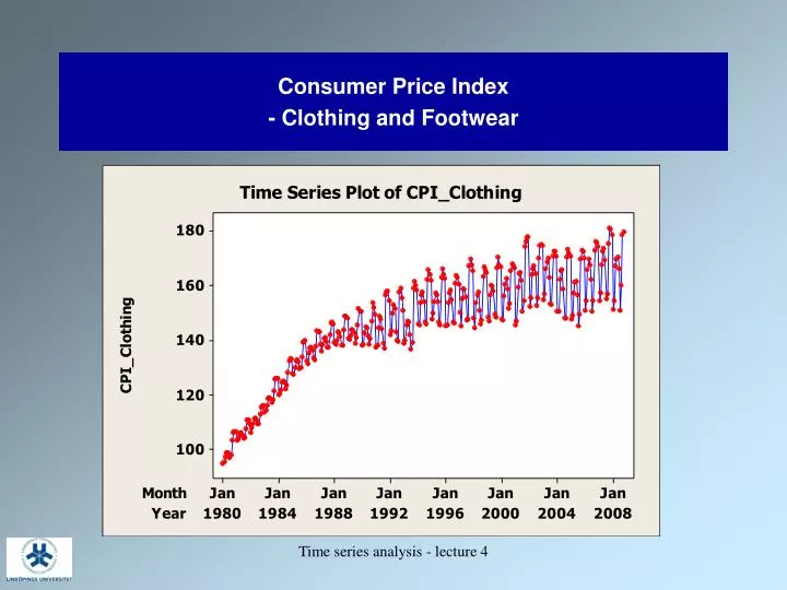
Consumer Price Index- Clothing and Footwear Time series analysis - lecture 4

Seasonally differenced Consumer Price Index- Clothing and Footwear Time series analysis - lecture 4

CPI Clothing and FootwearSARIMA (1, 0, 0, 0, 1, 0) Final Estimates of Parameters Type Coef SE Coef T P AR 1 0.7457 0.0522 14.29 0.000 Constant 0.2222 0.1783 1.25 0.214 Differencing: 0 regular, 1 seasonal of order 12 Number of observations: Original series 178, after differencing 166 Residuals: SS = 865.115 (backforecasts excluded) MS = 5.275 DF = 164 Time series analysis - lecture 4

CPI Clothing and FootwearSARIMA (1, 0, 0, 2, 1, 0) Final Estimates of Parameters Type Coef SE Coef T P AR 1 0.8145 0.0460 17.72 0.000 SAR 12 -0.6092 0.0830 -7.34 0.000 SAR 24 -0.2429 0.0843 -2.88 0.005 Constant 0.3275 0.1557 2.10 0.037 Differencing: 0 regular, 1 seasonal of order 12 Number of observations: Original series 178, after differencing 166 Residuals: SS = 651.883 (backforecasts excluded) MS = 4.024 DF = 162 Time series analysis - lecture 4

CPI Clothing and FootwearSARIMA (1, 0, 0, 2, 1, 0) residuals Time series analysis - lecture 4

Models for multiple time series of data • Dynamic regression models • General input-output models • Models for intervention analysis • Response surface methodologies • Smoothing of multiple time series • Change-point detection Time series analysis - lecture 4

Percentage of carbon dioxide in the output from a gas furnace Time series analysis - lecture 4

The dynamic regression model where Yt = the forecast variable (output series); Xt = the explanatory variable (input series); Nt = the combined effect of all other factors influencing Yt(the noise); (B) = (0 + 1B + 2B2 + … +kBk), wherekis the order of the transfer function Time series analysis - lecture 4

Using the SAS procedure AUTOREG- regression in which the noise is modelled as an autoregressive sequence Consider a dataset with one input variable (gasrate) and one output variable (CO2) data newdata; set mining.gasfurnace; gasrate1= lag1(gasrate); gasrate2= lag2(gasrate); gasrate3=lag3(gasrate); gasrate4= lag4(gasrate); run; procautoreg data=newdata; model CO2 = gasrate/nlag=1; model CO2 = gasrate gasrate1/nlag=1; model CO2 = gasrate gasrate1 gasrate2/nlag=1; model CO2 = gasrate gasrate1 gasrate 2 gasrate3/nlag=1; model CO2 = gasrate gasrate1 gasrate2 gasrate3 gasrate4/nlag=1; output out=model4 residual=res; run; Time series analysis - lecture 4

Predicted and observed levels of carbon dioxide in the output from a gas furnace- dynamic regression model with inputs time-lagged up to 4 steps Time series analysis - lecture 4

No. air passengers by week in Sweden-original series and seasonally differenced data Time series analysis - lecture 4

Intervention analysis where Yt = the forecast variable (output series); Xt = the explanatory variable (step or pulse function); Nt = the combined effect of all other factors influencing Yt(the noise); (B) = (0 + 1B + 2B2 + … + kBk), wherekis the order of the transfer function Time series analysis - lecture 4

Consumer Price Index - Clothing and Footwear