Download
1 / 22
220 likes | 338 Views
Hybrid quantum decoupling and error correction. University of California, Riverside. Leonid Pryadko. Yunfan Li (UCR) Daniel Lidar (USC). Pinaki Sengupta ( LANL ) Greg Quiroz (USC) Sasha Korotkov (UCR). Outline.

E N D
Hybrid quantum decoupling and error correction University of California, Riverside Leonid Pryadko Yunfan Li (UCR) Daniel Lidar (USC) Pinaki Sengupta (LANL) Greg Quiroz (USC) Sasha Korotkov (UCR)
Outline • Motivation: QEC and encoded dynamical decoupling with correlated noise • General results on dynamical decoupling • Concurrent application of logic • Intercalated application of logic • Conclusions and perspective
Stabilizer QECC • Error correction is done by measuring the stabilizers frequently and correcting with the corresponding error operators if needed • QECC period should be small compared to the decoherence rate • Traditional QECCs: • Expensive: need many ancillas, fast measurement, processing & correcting • May not work well with correlated environment
QECC with constant error terms [[3,1,3]] 1 qubit [[5,1,5]] [[5,1,3]]
QECC with constant error terms & decoupling [[5,1,5]]: fix 1- & 2-qubit phase errors Q2 1-qubit symmetric seq. X Y S1=XXIII, S2=IXXII, S3=IIXXI, S4=IIIXX [[5,1,3]] [[5,1,5]]
Combined coherence protection technique • Passive: Dynamical Decoupling • Effective with low-frequency bath • Most frugal with ancilla qubits needed • Needs fast pulsing (resource used: bandwidth) • Active: Quantum error correcting codes • Most universal • Needs many ancilla qubits • Needs fast measurement, processing & correcting • Expensive • Combined: Encoded Dynamical Recoupling [Viola, Lloyd & Knill (1999)] • Better suppression of decoherence due to slow environment potentially much more efficient • Control can be done along with decoupling
Example with hard pulses & constant errors • Errors are fully reversed at the end of the decoupling cycle • Normalizer and stabilizer commute – add logic anywhere!? 1 2 1 2 XLYLZL
Example with hard pulses & constant errors • Errors are fully reversed at the end of the decoupling cycle • Normalizer and stabilizer commute – add logic anywhere! 1 2 1 2 XLYLZL 1 2 XLYLZL
Error operators in rotating frame • S: system, E: environment, DD: dynamical decoupling • Dynamical decoupling is dominant: is large • Solve controlled dynamics and write the Hamiltonian in the interaction representation with respect to DD • Interaction representation with respect to environment • Bath coupling is now modulated at the combination of the environment and dynamical decoupling frequencies • With first-order average Hamiltonian suppressed, all S+E coupling is shifted to high frequences no T1 processes (Kofman & Kurizki, 2001)
Resonance shift with decoupling • Slowly-evolving system couple strongly to low- noise • Decoupling with period 2/ suppresses the low- spectral peak & creates new peaks shifted by n • Noise decoupling similar with lock-in techniques Environment spectrum F(w) system spectrum with refocusing |0i |1i ~ w W 2W
Resonance shift with decoupling • Slowly-evolving system couples strongly to low- noise • Decoupling with period 2/ suppresses the low- spectral peak & creates new peaks shifted by n • Noise decoupling similar with lock-in techniques Environment spectrum F(w) system spectrum with refocusing |0i |1i ~ w W 2W By analyticity, reactive processes should also be affected
Quantum kinetics with DD: results • K=0 (no DD): Dephasing rate 0» max(J,(0)0), (t)=||hB(t)B(0)i|| • K=1 (1st order): Single-phonon decay eliminated Dephasing rate 1» max(J2,(0)), plus effect of higher order derivatives of (t) at t=0. Reduction by factor /0 • K=2 (2nd order): all derivatives disappear Exponential reduction in /0 • Visibility reduction »(0)2 (generic sequence) »’’(0)4 »(0)4/t02 (symmetric sequence) (LPP & P. Sengupta, 2006)
Encoded dynamical recoupling • Several physical qubits logical • Operators from the stabilizer are used for dynamical decoupling ( ), at the same time running logic operators from • It is important that mutually commute (Viola, Lloyd & Knill,1999)
No-resonance condition for T1 processes mutually commute • Interaction representation • Combination of three rotation frequencies • Harmonics of DD (periodic) • L (can be small since logic is not periodic) • E (limited from above by Emax) • State decay through environment is suppressed if
No-resonance: spectral representation • DD pulses shift the system’s spectral weight to higher frequencies • Simultaneous execution of non-periodical algorithm widens the corresponding peaks • More stringent condition to avoid the overlap with the spectrum of the environmental modes Environment spectral function F(w) system spectrum with refocusing with DD & Logic w W 2W
Recoupling with concurrent logic 1 2 XLYLZL 4-pulse
Recoupling with concurrent logic: expand 1 2 XLYLZL 4-pulse L=4
Intercalated pulse application • Apply logical pulses at the end of the decoupling interval • With hard pulses, this cancels the average error over decoupling period [Viola et al, 1999] • Overlap with bath is power-law in c • Equivalently, visibility reduction with each logic pulse • With finite-length pulses, additional error depending on pulse duration and precise placement • Use shaped pulses to construct sequences with no errors to 1st or 2nd order Environment spectral function F(w) system spectrum with refocusing with DD & Logic w W 2W Power of ||
Recoupling with intercalated logic 1 2 XLYLZL 4-pulse
Recoupling with intercalated logic (cont’d) 1 2 XLYLZL 4-pulse
Compare at t/p=384 Concurrent Intercalated Concurrent Concurrent
Conclusions and Outlook • Much mileage can be gained from carefully engineered concatenation • With decoupling at the lowest level, need careful pulse placement, pulse & sequence design • Bandwidth is used to combine logic and decoupling • Still to confirm predicted parameter scaling • Analyze effects of: • Actual many-qubit gates needed • Fast decoherence addition • QEC dynamics (gates with ancillas, measurement,…) • Can fault-tolerance be achieved in this scheme?