Download
1 / 53
650 likes | 938 Views
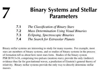
Binary Systems and Stellar Parameters.

E N D
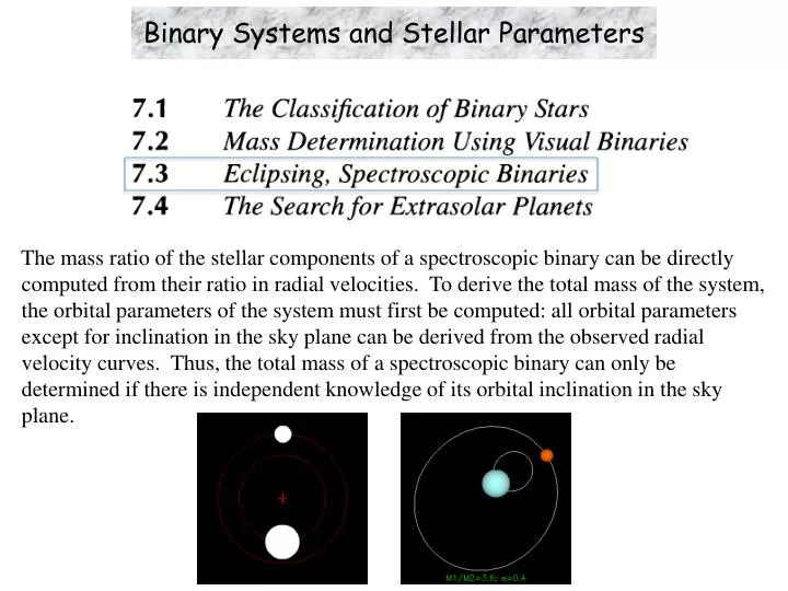
Binary Systems and Stellar Parameters The mass ratio of the stellar components of a spectroscopic binary can be directly computed from their ratio in radial velocities. To derive the total mass of the system, the orbital parameters of the system must first be computed: all orbital parameters except for inclination in the sky plane can be derived from the observed radial velocity curves. Thus, the total mass of a spectroscopic binary can only be determined if there is independent knowledge of its orbital inclination in the sky plane.
Learning Objectives • Non-Eclipsing Spectroscopic BinariesRadial-Velocity Curves Tidal Circularisation Total Mass Mass Ratio Individual Stellar Masses Mass Function • Eclipsing Spectroscopic BinariesLight Curves Total Mass Stellar Radii Stellar Effective Temperatures
Learning Objectives • Non-Eclipsing Spectroscopic BinariesRadial-Velocity Curves Tidal Circularisation Total Mass Mass Ratio Individual Stellar Masses Mass Function • Eclipsing Spectroscopic Binaries Light Curves Total Mass Stellar Radii Stellar Effective Temperatures
Spectroscopic Binary: Radial Velocity Curves • Consider a double-line spectroscopic binary with a circular orbit and its orbital plane perpendicular to the plane of the sky (i.e., observed edge-on, with i = 90°). • Doppler shift • At low speeds v« c, use the approximation and ignore terms (vr/c)2 to find observer
Spectroscopic Binary: Radial Velocity Curves • Consider a double-line spectroscopic binary with a circular orbit and its orbital plane perpendicular to the plane of the sky (i.e., observed edge-on, with i = 90°). • The measured radial velocity of each component will vary sinusoidally about the systemic velocity, vcm. (The systemic velocity is the overall radial velocity of the system with respect to us.) Thus, the observed radial velocity curve of each component is sinusoidal. max vr = vorb
Spectroscopic Binary: Radial Velocity Curves • Consider a double-line spectroscopic binary with a circular orbit, but now with its orbital plane inclined at an angle i to the plane of the sky. • The measured radial velocity of component 1 is v1r = v1 sin i, and that of component 2 is v2r = v2 sin i. How does this affect the observed radial velocity curve of each component? d i
Spectroscopic Binary: Radial Velocity Curves • Consider a double-line spectroscopic binary with a circular orbit, but now with its orbital plane inclined at an angle i to the plane of the sky. • The measured radial velocity of component 1 is v1r = v1 sin i, and that of component 2 is v2r = v2 sin i. The observed radial velocity curve of each component remains sinusoidal but now has a smaller amplitude (i.e., smaller maximum velocity). max vr = vorb sin i d i
Spectroscopic Binary: Radial Velocity Curves • Consider a double-line spectroscopic binary with an elliptical orbit and its orbital plane perpendicular to the plane of the sky (i.e., observed edge-on, with i = 90°). • The observed radial velocity curves are no longer sinusoidal, and furthermore depend on the orientation of the orbits (angle ω, argument of periastron) with respect to the observer as illustrated below for a single-line spectroscopic binary.
Spectroscopic Binary: Radial Velocity Curves • Consider a double-line spectroscopic binary with an elliptical orbit and its orbital plane perpendicular to the plane of the sky (i.e., observed edge-on, with i = 90°). • The observed radial velocity curves are no longer sinusoidal, and furthermore depend on the orientation of the orbits (angle ω, argument of periastron) with respect to the observer as illustrated below for a single-line spectroscopic binary. max vr = max vorb max vr ≠ max vorb
Spectroscopic Binary: Radial Velocity Curves • Consider a double-line spectroscopic binary with an elliptical orbit and its orbital plane perpendicular to the plane of the sky (i.e., observed edge-on, with i = 90°). • The observed radial velocity curves are no longer sinusoidal, and furthermore depend on the orientation of the orbits (angle ω) with respect to the observer as illustrated below for a double-line spectroscopic binary with e = 0.4 and ω = 45°. • How would the radial velocity curves change if the orbit is not in the plane of the sky?
Spectroscopic Binary: Radial Velocity Curves • Consider a double-line spectroscopic binary with an elliptical orbit and its orbital plane perpendicular to the plane of the sky (i.e., observed edge-on, with i = 90°). • The observed radial velocity curves are no longer sinusoidal, and furthermore depend on the orientation of the orbits (angle ω) with respect to the observer as illustrated below for a double-line spectroscopic binary with e = 0.4 and ω = 45°. • If i ≠ 90°, shape remains the same but amplitudes of the observed radial velocity curves decrease.
Spectroscopic Binary: Radial Velocity Curves • Each combination of ω and e produces a radial velocity curve with a different shape. Thus, ω and e can be determined from the shape of the observed radial velocity curve, and therefore also projected orbital velocity, vorb sin i, and, of course, orbital period, P. max vr = max vorb max vr ≠ max vorb
Spectroscopic Binary: Radial Velocity Curves • Measurements of radial velocity curves of spectroscopic binaries in the open cluster Blanco 1 (González & Levato 2009, A&A, 507, 541). P = 1740 days P = 2.4 days P = 51.4 days P = 191.4 days P = 2.4 days P = 5.4 days P = 1338 days P = 1.9 days
Learning Objectives • Non-Eclipsing Spectroscopic BinariesRadial-Velocity Curves Tidal CircularisationTotal Mass Mass Ratio Individual Stellar Masses Mass Function • Eclipsing Spectroscopic Binaries Radial-Velocity Curves Total Mass Stellar Radii Stellar Effective Temperatures
Tidal Circularization of Binary Systems • A binary system is more likely to be detected as a spectroscopic binary if its orbital period is short, and hence if the two stellar components are closely separated (and/or massive). The orbits of tight binary systems circularize rapidly due to tidal forces between the two stars.
Learning Objectives • Non-Eclipsing Spectroscopic BinariesRadial-Velocity CurvesTidal CircularisationTotal Mass Mass Ratio Individual Stellar Masses Mass Function • Eclipsing Spectroscopic Binaries Radial-Velocity Curves Total Mass Stellar Radii Stellar Effective Temperatures
Spectroscopic Binary: Total Mass • The total mass of a spectroscopic binary can be determined from Kepler’s 3rd law • Replacing the semimajor axis of the reduced mass system, a, with (at focus of ellipse) a
Spectroscopic Binary: Total Mass • The total mass of a spectroscopic binary can be determined from Kepler’s 3rd law • Replacing the semimajor axis of the reduced mass system, a, with a1 a2
Spectroscopic Binary: Total Mass • The total mass of a spectroscopic binary can be determined from Kepler’s 3rd law • Replacing the semimajor axis of the reduced mass system, a, with • (which does not require knowing the distance to the system) and solving for the total mass • in the case where i = 90°. Unlike visual binaries, determining the total mass of the binary system does not require knowing the distance to the system.
Spectroscopic Binary: Total Mass • The total mass of a spectroscopic binary can be determined from Kepler’s 3rd law • Replacing the semimajor axis of the reduced mass system, a, with • (which does not require knowing the distance to the system) and solving for the total mass • in the case where i ≠ 90° so that and . The total mass of spectroscopic binaries can therefore be determined only if the orbital inclination is known. How do we determine the inclination of the orbits of spectroscopic binaries?
Spectroscopic Binary: Total Mass • The total mass of a spectroscopic binary can be determined from Kepler’s 3rd law • Replacing the semimajor axis of the reduced mass system, a, with • (which does not require knowing the distance to the system) and solving for the total mass • in the case where i ≠ 90° so that and . The total mass of spectroscopic binaries can therefore be determined only if they also are visual binaries or eclipsing systems, making such systems especially valuable for precise determinations of stellar masses.
Learning Objectives • Non-Eclipsing Spectroscopic Binaries Radial-Velocity Curves Tidal CircularisationTotal Mass Mass Ratio Individual Stellar Masses Mass Function • Eclipsing Spectroscopic Binaries Radial-Velocity Curves Total Mass Stellar Radii Stellar Effective Temperatures
Spectroscopic Binary: Mass Ratio • For a spectroscopic binary with a circular or a very small eccentricity (e « 1) orbit, the orbital velocities of the two component are (nearly) constant and given by • Unlike in the case of visual binaries, the orbital semimajor axis of the individual components can be determined from the orbital measurements alone. • From Eq (7.1) • we find • in the case where i = 90° (edge-on orbit). to Earth
Spectroscopic Binary: Mass Ratio • For i ≠ 90°, the observed radial velocities • and hence from Eq. (7.4) the mass ratio • Like for visual binaries, the mass ratio can be determined without knowing the orbital inclination. Unlike for visual binaries (where the location of the center of mass must be determined), the mass ratio can be determined from the orbital measurements alone. As radial velocities can usually be measured to higher precision than astrometric measurements of the system’s center of mass, the mass ratio of spectroscopic binaries can usually be determined to a higher precision than that of visual binaries (which are not also spectroscopic binaries). to Earth to Earth
Learning Objectives • Non-Eclipsing Spectroscopic Binaries Radial-Velocity Curves Tidal Circularisation Total Mass Mass Ratio Individual Stellar Masses Mass Function • Eclipsing Spectroscopic Binaries Radial-Velocity Curves Total Mass Stellar Radii Stellar Effective Temperatures
Spectroscopic Binary: Total Mass • By deriving the mass ratio (which does not require knowing the orbital inclination) • and total mass of the system (which requires knowing the orbital inclination) • the masses of the individual components can be derived. • Even if orbital inclinations are not known, the total masses of spectroscopic systems can be estimated statistically by assuming that ‹sin3i› ≈ 2/3. By grouping stars according to their effective temperatures or luminosities (if their distances are known), any dependence of these quantities on stellar mass can be studied.
Mass-Luminosity Relationship of Stars • In this way, astronomers have established that the luminosity of a main-sequence star depends on its mass.
Learning Objectives • Non-Eclipsing Spectroscopic Binaries Radial-Velocity Curves Tidal Circularisation Total Mass Mass Ratio Individual Stellar Masses Mass Function • Eclipsing Spectroscopic Binaries Radial-Velocity Curves Total Mass Stellar Radii Stellar Effective Temperatures
Spectroscopic Binary: Mass Function • For a single-line spectroscopic binary (i.e., where one component is so much brighter than the other that the dimmer component is not detectable), P = 1740 days P = 2.4 days P = 51.4 days P = 191.4 days P = 2.4 days P = 5.4 days P = 1338 days P = 1.9 days
Spectroscopic Binary: Mass Function • For a single-line spectroscopic binary (i.e., where one component is so much brighter than the other that the dimmer component is not detectable), we replace v2r in the expression for the total mass given by Eq. (7.6) • by its expression for the mass ratio as given by Eq. (7.5) • to give
Spectroscopic Binary: Mass Function • Rearranging, we get • The RHS of Eq. (7.7), which depends only on the observable quantities P and v1r, is known as the mass function. Mass function is particularly useful if an estimate of the mass of the visible star by some indirect means already exists, otherwise useful only for statistical studies • Note that • If either m1 or sin i is, or both are, unknown, the mass function sets a lower limit for m2, the mass of the undetectable secondary component. As we shall see, this is especially pertinent when deriving the masses of extrasolar planets. <
Learning Objectives • Non-Eclipsing Spectroscopic Binaries Radial-Velocity CurvesTidal Circularisation Total Mass Mass Ratio Individual Stellar Masses Mass Function • Eclipsing Spectroscopic BinariesLight Curves Total Mass Stellar Radii Stellar Effective Temperatures
Eclipsing Spectroscopic Binary • As mentioned earlier, the total mass of spectroscopic binaries can only be determined if these systems also are visual binaries or eclipsing systems. • Eclipsing spectroscopic binaries are especially valuable as they permit the simultaneous determination of stellar mass, radius, and if their distances are known, effective temperature and hence luminosity. (Although some stars are large enough for their radii to be measured using interferometry, the masses of these stars cannot be directly determined unless they belong to binary systems.)
Eclipsing Spectroscopic Binary: Inclination • For one star to eclipse another, the orbital plane must be close or exactly perpendicular to the plane of the sky (i.e., i ≈ 90°). This is much more likely if the two stars are closely separated: eclipsing binary systems are therefore quite likely to have circular or only weakly-eccentric orbits due to tidal circularization.
Eclipsing Spectroscopic Binary: Light Curves • The orbital inclination can be further constrained from the shape of the eclipse light curve. • If the light curve during eclipse exhibits a constant minimum, the orbital inclination must be almost exactly if not exactly 90°.
Eclipsing Spectroscopic Binary: Light Curves • The orbital inclination can be further constrained from the shape of the eclipse light curve. • If the light curve during eclipse does not exhibit a constant minimum, the orbital inclination must differ significantly from 90°.
Eclipsing Spectroscopic Binary: Light Curves • Example light curves of eclipsing binary systems. Note that, in general, the two dips in each light curve have different depths. Why?
Eclipsing Spectroscopic Binary: Light Curves • Example light curves of eclipsing binary systems. Note that, in general, the two dips in each light curve have different depths. Why?
Eclipsing Spectroscopic Binary: Light Curves • Example light curves of eclipsing binary systems. Note that, in general, the two dips in each light curve have different depths. Why? The two binary components have different effective temperatures.
Learning Objectives • Non-Eclipsing Spectroscopic Binaries Radial-Velocity CurvesTidal Circularisation Total Mass Mass Ratio Individual Stellar Masses Mass Function • Eclipsing Spectroscopic BinariesLight Curves Total Mass Stellar Radii Stellar Effective Temperatures
Eclipsing Spectroscopic Binary: Total Mass • The mass ratio of a spectroscopic binary can be determined without knowing the orbital inclination • The total mass of a spectroscopic binary can only be determined if the orbital inclination is known • For an eclipsing system, the orbital inclination must be quite close to 90° (unless the orbital separation is small compared to the stellar radii). For such systems, the error introduced by the uncertainty in orbital inclination is small: e.g., if i = 75° instead of i = 90°, the error introduced in determining m1 + m2 is only 10%.
Learning Objectives • Non-Eclipsing Spectroscopic Binaries Radial-Velocity CurvesTidal Circularisation Total Mass Mass Ratio Individual Stellar Masses Mass Function • Eclipsing Spectroscopic BinariesLight Curves Total Mass Stellar Radii Stellar Effective Temperatures
Eclipsing Spectroscopic Binary: Stellar Radii • Consider an eclipsing binary with a (nearly) circular orbit, an orbital plane at an inclination i ≅ 90°, and the semimajor axis of the smaller star’s orbit that is large compared to either star’s radius so that the smaller star is moving perpendicular to the observer’s line of sight during the duration of the eclipse. • The radius of the smaller star vs + vl (vs = velocity of small star, vl = velocity of large star)
Eclipsing Spectroscopic Binary: Stellar Radii • Consider an eclipsing binary with a (nearly) circular orbit, an orbital plane at an inclination i ≅ 90°, and the semimajor axis of the smaller star’s orbit that is large compared to either star’s radius so that the smaller star is moving perpendicular to the observer’s line of sight during the duration of the eclipse. • The radius of the larger star vs + vl (vs = velocity of small star, vl = velocity of large star)
Learning Objectives • Non-Eclipsing Spectroscopic Binaries Radial-Velocity CurvesTidal Circularisation Total Mass Mass Ratio Individual Stellar Masses Mass Function • Eclipsing Spectroscopic BinariesLight Curves Total Mass Stellar Radii Stellar Effective Temperatures
Eclipsing Spectroscopic Binary: Stellar Effective Temperatures • The surface flux (energy per unit time per unit area at the surface) of a blackbody is given by (see Chap. 3 of textbook) • As the same total cross-sectional area is eclipsed no matter whether the smaller star passes behind or in front of the larger star, the dip in the light is deeper (primary minimum) when the hotter star is eclipsed. In this case, which is the hotter star? σ = 5.670 x 10⁻⁸ W m-2 K-4 (Stefan-Boltzmann’s constant) secondaryminimum primary minimum
Eclipsing Spectroscopic Binary: Stellar Effective Temperatures • The surface flux (energy per unit time per unit area at the surface) of a blackbody is given by (see Chap. 3 of textbook) • As the same total cross-sectional area is eclipsed no matter whether the smaller star passes behind or in front of the larger star, the dip in the light is deeper (primary minimum) when the hotter star is eclipsed. In this case, which is the hotter star? The smaller star. σ = 5.670 x 10⁻⁸ W m-2 K-4 (Stefan-Boltzmann’s constant) secondaryminimum primary minimum
Eclipsing Spectroscopic Binary: Stellar Effective Temperatures • The surface flux (energy per unit time per unit area at the surface) of a blackbody is given by (see Chap. 3 of textbook) • As the same total cross-sectional area is eclipsed no matter whether the smaller star passes behind or in front of the larger star, the dip in the light is deeper (primary minimum) when the hotter star is eclipsed. In this case, which is the cooler star? σ = 5.670 x 10⁻⁸ W m-2 K-4 (Stefan-Boltzmann’s constant) secondaryminimum primary minimum
Eclipsing Spectroscopic Binary: Stellar Effective Temperatures • The surface flux (energy per unit time per unit area at the surface) of a blackbody is given by (see Chap. 3 of textbook) • As the same total cross-sectional area is eclipsed no matter whether the smaller star passes behind or in front of the larger star, the dip in the light is deeper (primary minimum) when the hotter star is eclipsed. In this case, which is the cooler star? The bigger star. σ = 5.670 x 10⁻⁸ W m-2 K-4 (Stefan-Boltzmann’s constant) secondaryminimum primary minimum
Eclipsing Spectroscopic Binary: Stellar Effective Temperatures • Assuming for simplicity that each star is uniformly bright across its disk, the amount of light detected outside eclipse • where k is a constant that depends on the distance to the binary system, amount of absorption by the medium between the star and telescope, and the efficiency of the telescope/detector (which can be characterized). surface flux of larger star surface flux of smaller star secondaryminimum primary minimum