Download
1 / 18
180 likes | 189 Views
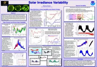
Solar Irradiance Variability. Claus Fröhlich, PMOD/WRC, Davos Dorf, Switzerland. Introduction TSI Measurements from space What about degradation What corrections are needed Development of a TSI Composite Construction of a composite Time series and Power Spectrum

E N D
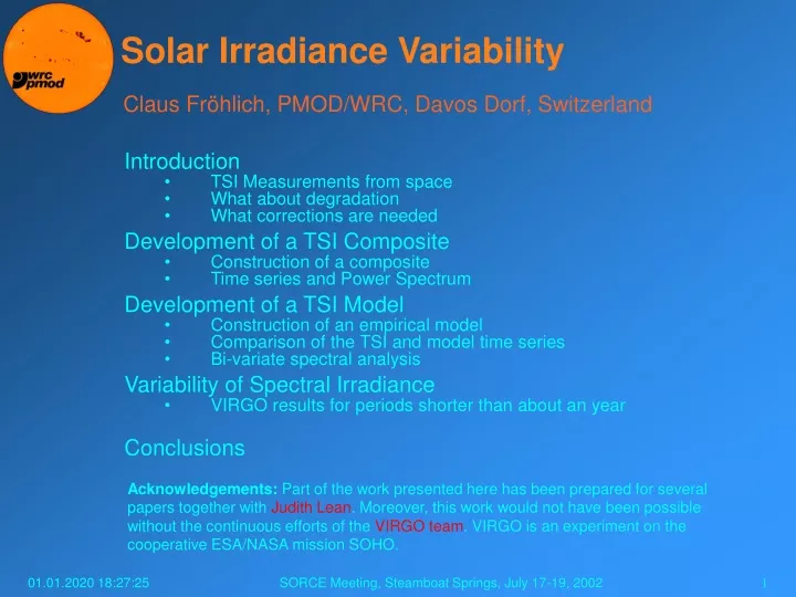
Solar Irradiance Variability Claus Fröhlich, PMOD/WRC, Davos Dorf, Switzerland Introduction • TSI Measurements from space • What about degradation • What corrections are needed Development of a TSI Composite • Construction of a composite • Time series and Power Spectrum Development of a TSI Model • Construction of an empirical model • Comparison of the TSI and model time series • Bi-variate spectral analysis Variability of Spectral Irradiance • VIRGO results for periods shorter than about an year Conclusions Acknowledgements: Part of the work presented here has been prepared for several papers together with Judith Lean. Moreover, this work would not have been possible without the continuous efforts of the VIRGO team. VIRGO is an experiment on the cooperative ESA/NASA mission SOHO. SORCE Meeting, Steamboat Springs, July 17-19, 2002
TSI Measurements from Space Total solar irradiance (TSI) monitoring from space with electrically calibrated radiometers started with the launch of NIMBUS-7 in November 1978 Several time series exist from different platforms made by different radiometers: HF on NIMBUS-7, ACRIM I on SMM, ERBE on ERBS, ACRIM II on UARS, VIRGO on SOHO and ACRIM III on ACRIMSat This allows the construction of a composite time series having improved long-term precision, thus yielding an unbiased estimate of TSI and its variability during the last almost three solar cycles For the discussion of the reliability of the composite mainly two issues are important: the correction for the early measurements of HF on NIMBUS 7 to account for its degradation and the tracing of ACRIM II to ACRIM I by comparison with ERBE and HF over the gap between them SORCE Meeting, Steamboat Springs, July 17-19, 2002
What about Degradation What can be learned from the VIRGO record? • Level-1 data • Transfer from ground to space • PMO6V shows ‘normal’ degradation as during earlier missions (ca. 2 ppm/day) • DIARAD is different and shows much smaller changes than before. The DIARAD-R seems to have more noise • PMO6V show an early increase which seem to be typical for these type of radiometers (as HF and possibly ACRIM-II) SORCE Meeting, Steamboat Springs, July 17-19, 2002
What about Degradation What can be learned from the VIRGO record: • Accurate assessment of degradation • Determination of non-exposure dependent changes • Correction of exposure dependent changes by comparison with less exposed radiometer of the same type • Comparison of the two type of radiometer, PMO6-V and DIARAD • Relative difference is repeated for after 1014 days more than 2 years • Conclusion: PMO6V does not show degradation other than due to exposure, DIARAD does (mainly during recovery after switch-off SORCE Meeting, Steamboat Springs, July 17-19, 2002
What Corrections are needed? Corrections of HF • Early increase and long-term degradation • Glitches in October 1989 and August 1990 • Lee et al., 1995, Chap-man et al. 1996 found 2 glitches of 0.36 and 0.37 W/m2 • Comparison of HF with ERBE and a model shows indeed a sudden change of HF after a 4-day switch-off. It is deter-mined as 0.42 W/m2. • The second glitch (at the vertical dashed line) is not confirmed, but a gra-dual change. • With the glitch correccted and the trend removed both the yield a horizon-tal line with a slope of -0.001 and -0.031 ppm/d for HF/ERBE and HF/model respectively SORCE Meeting, Steamboat Springs, July 17-19, 2002
What Corrections are needed? • How to refer ACRIM-II to the ACRIM-I scale? • Comparison with ERBE and HF before and after the gap • Obviously, the result depends on the corrections of HF • As the ration HF/ERBE has already been corrected the ACRIM-I to ACRIM-II reference does no longer really depend on whether one does it against ERBE or HF • There may be still some other periods in the HF record which needs corrections, as e.g. in 1987 as seen in the ACRIM/HF and HF/ERBE • It is interesting to note that ERBE shows also some early increase which seems to be finished by 1989 • These comparison show that in general the long-term behavior seems to be more robust than the short-term. SORCE Meeting, Steamboat Springs, July 17-19, 2002
Construction of the Composite • The reference in terms of absolute SI units is ACRIM-II, referred to SARR (Crommelynck et al., 1995) • The horizontal lines at zero indicate the use of the time series as they are (for VIRGO and ACRIM-I slightly shifted to match the record before) • HF seems to have an overall increase in sensitivity. It is interesting to note the trend determined by comparison with ACRIM-I in 82/82 is the same as the one determined from the comparison with ERBE during 89/92 as indicated by the dotted line • Looking at the ERBE data between 89/92 the issue of bridging the gap between ACRIM-I and ACRIM-II may still not be finalized SORCE Meeting, Steamboat Springs, July 17-19, 2002
Discussion of the composite TSI Time series • The solar cycle amplitude amounts to about 0.1% • Cycle 21 is the highest (could be due to the early HF correction – may have to be revisited) • Long-term trend as indicated by the difference between the two minima 21/22 and 22/23 amounts to 65.8 ppm, with the latter being lower. This corresponds to 6.29 ppm/a. This value depends mainly on the HF correction which is with 27.6 ppm/a quite uncertain. • How accurate is this trend? From comparison with ERBE and ACRIM-II and III when they are not part of the composite, a formal uncertainty about 3 ppm/a is deduced • The observed trend is with a high probability (about 2-3) not different from zero. SORCE Meeting, Steamboat Springs, July 17-19, 2002
Discussion of the composite TSI • Power Spectrum • The most interesting features are: • There is a broad peak around an 11-year period with essentially all the variance • There is a large dip at about 1450 days (about 4 years). Its origin is unknown. • There is a broad peak around 1 year, probably due to different activity levels in the N and S hemispheres • TSI has only little power at the 27-day rotational period. A factor of 2 less than above or below. • The spectrum is flat between about 4 years and 15 days. Below 15 days it decreases with about 1/f3. • The basis for the model used here comes next. Here we note that simulates quite well the TSI spectrum SORCE Meeting, Steamboat Springs, July 17-19, 2002
Development of an empirical model How do magnetic fields influence the irradiance? • TSI is only marginally correlated with global magnetic fields (absolute and average) • The effect of magnetic fields on irradiance is through changes of the temperature structure of the solar atmosphere • These changes can be monitored by e.g. the MgII index, the core-to-wing intensity ratio SORCE Meeting, Steamboat Springs, July 17-19, 2002
Development of an empirical model The model is based on sunspot darkening and brightening by faculae and network • The influence of sunspots on the irradiance, F0, is modeled by the Photometric Sunspot Index PS • For the facular influence a similar index, PF can be determined. How-ever, it depends on the availability of images. Here we model the influence of faculae and network PF by the MgII index which corresponds to the core-to-wing intensity ratio of the Mg line at 280 nm. Moreover, we separate PF in a long- and short-term part. The former represents the faculae, the latter the network • These three components, PS , PFs and PFl are calibrated by multiple linear regression against TSI. SORCE Meeting, Steamboat Springs, July 17-19, 2002
Comparison of TSI with the Model The Camel/Dromedary approach • In contrast to sunspots faculae exhibit a CLV which substantially different from the photospheric one. • The effect of sunspots peaks at the central meridian passage where they are darkest. As faculae and network show limb brightening they influence the irradiance (different for luminosity) with two peaks around the central meridian passage separated by about 8-10 days • As the irradiance, corrected for sunspots, F0+PS,, shows a double peak this time series is convoluted with a double-peak filter (Camel), whereas PFs with a triangular one (Dromedary). • The Camel filter is optimized for the highest correlation between the filtered F0+PS and PFs , time series. SORCE Meeting, Steamboat Springs, July 17-19, 2002
Comparison of TSI with the Model • The correlation seems to be quite good for the different periods although the correlation is calculated with all data. • The model for the maximum of cycle 21 is too low, and about right for the maxima of 22 and 23. In general the short-term variation seems to be underestimated. It is most obvious in cycle 23 with less sunspots. It is interesting to note that factor for PFs is about 2/3 of the one for PFl. • The correlation with 0.916 tells us that 84% of the variance is explained Time Series SORCE Meeting, Steamboat Springs, July 17-19, 2002
Comparison of TSI with the Model Difference between Cycles and Long-term Trends • The three cycles are quite different, especially the ascending part of 22 and 23. For the latter it could be that a first maximum was already reached in late 1998. • The residual shows a down-ward trend of 8.8 ppm/a which is close to the 6.3 ppm/a found from the difference of TSI at the two minima 21/22 and 22/23. SORCE Meeting, Steamboat Springs, July 17-19, 2002
Comparison of TSI with the model Bi-variate spectral analysis • The bi-variate spectral analysis calculates as a function of frequency a filter which trans-forms – in our case – the model into TSI. • The association is quantified by the coherence . 1002 gives the amount explained in percent. • High values with 2>0:94 are reached at periods around 295, 103, 31 and 24 days and low ones 2< 0:20 at periods around 198, 80, 69, 28, 19 and <8 days. • The average gain and phase over the range of periods from 13 to 1200 days amount to 1.02 and -1 deg; respectively which confirms the regression results. SORCE Meeting, Steamboat Springs, July 17-19, 2002
Variability of Spectral Irradiance SPM VIRGO time series • For detrending the level-1 SPM, the combination of the operational (a) and the backup (b) cannot be used in the same way as for the radiometers. • The back-up (panel b) behave in an rather unexpected way which is a combination of the solar and still not identified instrumental changes. • A polynomial fit to the ratio of (a) to (b) for each channel allows to construct detrended time series which allow to study solar variability up to periods of about one year. SORCE Meeting, Steamboat Springs, July 17-19, 2002
Variability of Spectral Irradiance Multi-variate spectral analysis • The total coherence is quite high. The share between the three channels is varying with frequency • At the rotational frequency the blue and green are less contributing than the red. This is even more pronounced at the 13-day period • The gain indicates that the ratio of the three colors to the total is about 1.8, 2.3 and and 4.1 for red/green/blue respectively • The results for the phase are difficult to interpret as they are quite uncertain. SORCE Meeting, Steamboat Springs, July 17-19, 2002
Conclusions • The solar cycle variation has an amplitude of about 0.1%. The three cycles as observed are still different – with more measurements we may eventually understand these differences. • A long-term trend is determined by comparison the two minima between 21/22 and 22/23 with 6.3 ppm/a. It is, however, mainly determined by how TSI is determined during the gap between ACRIM-I and II. The trend is not significantly different from zero and we are still not able to detect a long-term trend. • 86% of the TSI variability can be explained by a 3-component model (sunspots: PS, MgII index: PFs and PFl). A linear fit to the residual shows a downward trend of 8.8 ppp/a which is obviously due to TSI and not the model. • SPM/VIRGO time series provide information about the spectral redistribution during changes of TSI. These results demonstrate the importance of continuous time series of spectral irradiance such as SIM will provide with SORCE SORCE Meeting, Steamboat Springs, July 17-19, 2002