Download
1 / 18
180 likes | 308 Views
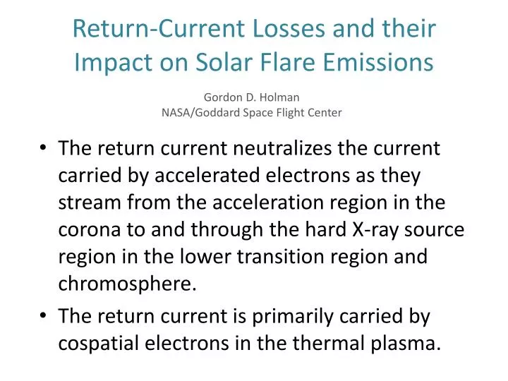
Return-Current Losses and their Impact on Solar Flare Emissions. Gordon D. Holman NASA/Goddard Space Flight Center.

E N D
Return-Current Losses and their Impact on Solar Flare Emissions Gordon D. HolmanNASA/Goddard Space Flight Center • The return current neutralizes the current carried by accelerated electrons as they stream from the acceleration region in the corona to and through the hard X-ray source region in the lower transition region and chromosphere. • The return current is primarily carried by cospatial electrons in the thermal plasma.
Why is the Return Current Important? • It allows the electron beam to exist. • It resupplies electrons to the acceleration region. • It directly heats the coronal part of flare loops. • The induced electric field that drives the return current also decelerates the streaming, accelerated electrons. This modifies the electron distribution and, therefore, the hard X-ray emission.
Purpose of this Work • To better understand the impact of return-current losses on solar flare hard X-ray emission • Extend earlier work by Knight & Sturrock (1977), Emslie (1980), Diakonov & Somov (1988), andLitvinenko & Somov (1991) to derive relatively simple analytic expressions for return-current losses alone for comparison with results from more elaborate numerical simulations obtained by Zharkova & Gordovskyy (2006) – “ZG06”
Properties of the ZG06 Electron Distribution Function • Single power law • Low-energy cutoff: ELC = 8 keV • High-energy cutoff: EHC = 384 keV • Pitch angle distribution exp{[( 1)/]2},where is the pitch angle cosine and = 0.2 The electron distribution is exp{25} smaller at 90 pitch angle than at 0. Therefore, a 1-D model should be adequate.
One-Dimensional Model • Assumptions: • Injectedsingle-power-lawelectron flux density distribution (electrons s-1 cm-2 keV-1)F(E, x=0) = (-1)Ec-1Fe0Ewith low-energy cutoffEc. • Steady state, return-current electric field strengthE = J, where is the classical (collisional) resistivity and J(x) is the current density. • J(x) = eFe(x), where Fe(x) = is the total beam electron flux density(electrons s-1 cm-2). • Electrons are lost from the beam when E = Eth = kBT, where T is the ambient plasma temperature.
Results • The electron flux density distribution at position x is F(E,x) = (-1)Ec-1Fe0[E+V(x)]above a cutoff at Max{Eth, EcV(x)}. V(x) = is the potential drop at distance x. Thus, V(x) behaves as a new low-energy cutoff to the flux density distribution, increasing with distance x. • The effective cutoff energy does not increase above Ec until the critical distancexrc = (Ec Eth)/(eErc0), where Erc0 = eFe0 is the electric field strength at x = 0 and Fe0 is the total injected electron flux density. Below xc the total electron flux densityis constant (Fe(x) = Fe0 for x ≤ xc).
1-D Results (continued) • For x >> Ec/(δeErc0), Fe(x) = Fe0[(δeErc0/Ec)x](δ-1)/ δ • Since the resistivity constant T3/2, until collisional losses become important the return current losses are not sensitive to the plasma density. • Electron energy as a function of distance isE(x) = E0 V(x). Therefore, all electrons lose the same amount of energy with distance x. For x ≤ xrc , V(x) = eErc0xFor x >> Ec/(δeErc0), V(x) = Ec[(δeErc0/Ec)x]1/ δ
More about the Return-Current Electric Field Strength Return-current losses decrease at the same time the electric field is having its greatest impact on the electron distribution, since the electric field strength is proportional to the total nonthermal electron flux density. Other losses to the electron distribution, including collisional losses and, in a 2-D model, the scattering of electrons through 90 pitch angle, also decrease the return-current electric field strength. Erc0 The figure on the right shows the typical change in the electric field strength with distance in the 1-D model with return-current losses only (blue curve) and for an initially isotropic electron pitch angle distribution (red curve). xrc
Return-Current Electric Field Strength from Zharkova & Gordovskyy 2006 (ZG06), Fig. 1 = 3 = 7 • The electric field strength is normalized to the Dreicer field, ED = 2e3n ln / (kBT). • It is plotted against column density, N(x) = n(x)dx. • The dashed curve is for an electron power-law index of 3 and the solid curve is for an index of = 7. • Results for three initial electron beam energy flux densities Pe0are shown: a) 108, b)1010, and c) 1012 erg cm-2 s-1. 108 erg cm-2 s-1 3 7 1010 erg cm-2 s-1 1012 erg cm-2 s-1 7 3
Modeling the ZG06 Electric Field Results • The 1-D model is applied since (1) the electron distribution is exp{25} smaller at 90 pitch angle than at 0 and (2) the electric field structure vs. column density computed by ZG06 shows the sharp drop off characteristic of the 1-D model. • Collisional losses should affect the electric field strength at column densities N Ec2/2K 82/(6 10-18) = 1 1019 cm-2. The results in panel (c) are modeled with return-current losses only since the evolution before N = 1019 cm-2 should be unaffected by collisional losses. • From Fig. 1c, Nrcnxrc 1 1018 cm-2 and Erc/ED 150. These two equations together determine the plasma density n and temperature T. For Eth 0, no solution could be found! Setting Eth = 0, these equations give T = 600 MK and n = 7 107 cm-3, extreme values, even for the flaring corona!
Comparison of Analytical and Numerical Models for E/ED Pe0 = 1012 erg cm-2 s-1 In the analytical model, n & T are taken to be constant withn = 7 107 cm-3 & T = 600 MK. 3 7 7 3 Nrc 7 3
Comparison of Analytical and Numerical Models for E/ED Pe0 = 1012 erg cm-2 s-1 Exponential downward increase in density, decrease in temperature. n0 = 7.5 107 cm-3 T0 = 3,000 MKLn = 1 1010 cmLT = 3 109 cm 3 7 7 3 Nrc 7 3
X-ray Spectra Comparison of Computed Spectra with ZG06 The Electron Distribution Function • 1-D model • Assume V(x) is approximately constant in the thick-target emission region ( VTT). This is likely to be correct for case (c) addressed above (Pe0 = 1012 erg cm-2 s-1).
Pe0 = 1012 erg cm-2 s-1 Comparison of Computed Spectra with ZG06 • = 7 • VTT = 14 keV • = 3 • VTT = 130 keV Thick-target bremsstrahlung spectra computed with F(E) (E+VTT), normalized to the flux at 4 keV. These are compared to spectra from Fig. 10b of ZG06 for = 3 (diamonds) and = 7 (squares). The best fits to the ZG06 spectra determined the values for VTT.
Interpretation of the Spectral Results • The spectra from the numerical model of ZG06 are will fitted by the spectra computed from the 1-D analytical model at and below 100 keV. • Agreement is not good above 100 keV, however, especially for = 3. The spectrum for = 3 falls off rapidly above 100 keV in the analytical model because the value of V is high in the thick-target region, where the high-energy cutoff has decreased to 384 keV – 130 keV = 254 keV. The ZG06 spectrum does not show a cutoff significantly below the initial value of 384 keV. • This decrease in the value of the high-energy cutoff with increasing potential drop V qualitatively explains why the spectral index at 100 keV becomes somewhat larger as the value of Pe0 increases (seen in Fig. 11 of ZG06).
Spectra and Spectral Indicesfrom ZG06 = 3 high low = 7 108 1010 Pe0 = 108erg cm-2 s-1 1012erg cm-2 s-1 20 keV = 7 100 keV = 5 = 3 Pe0 = 1012 erg cm-2 s-1
Potential Drop V vs. Column Density Nfrom the 1-D Model with Constant n & T 384 keV EHC 130 keV VTT( = 3) Large difference in VTT for = 3 = 3 = 7 14 keV VTT( = 7) ELC 8 keV CollisionalLosses Thick-Target Region
Conclusions • The simple analytical model does an excellent job of explaining the qualitative features of return-current losses. • Substantial quantitative differences between the analytical and numerical model results indicate that quantitative comparisons of simplified numerical model computations with analytical and semi-analytical model results now need to be pursued.